Estimating fractional cover

Learning goals

Understand the basic concept of linear spectral unmixing and generation of synthetic training data
Use Support Vector Regression (SVR) models and Random Forest Regression (RFR) to estimate fractional cover of photosynthetic vegetation (PV), non-photosynthetic vegetation (NPV) and soil for agricultural fields in northeastern Germany.
Evaluate fractional cover estimates from Sentinel-2 with reference fractional cover

Background

The mixed pixel problem

In this course, you have already learned how to make use of multispectral data to generate land cover maps. However, you may have noticed that often a pixel contains more than one cover type. This happens when the land cover is heterogeneous on the sub-pixel scale. Classification approaches assign discrete labels to a pixel and can thus be of limited use for estimating the true distribution of a surface material. In many cases (but very much depending on the training dataset), the dominant class label will be assigned by the classification model. We thereby underestimate the proportion(s) of the minority class(es), while overestimating the proportion of the dominant class.

A good example are urban areas, where e.g. rooftops, streets and single trees fall within a single Sentinel-2 or Landsat pixel. On agricultural fields, pixels often contain mixtures of photosynthetically active vegetation, dead plant material (e.g. litter or standing dead biomass) and open soil. As the cover quantities vary over time on croplands, we can use fractional cover to better understand the vegetation changes in response to e.g. land management and weather extremes.

Fig. by Ali et al. (2016) DOI: 10.1093/jpe/rtw005

With fraction mapping we attempt to map the fraction of a variety of classes within a pixel. This can either be done by using spectral mixture analysis or regression approaches.

Spectral unmixing with regression models

Instead of assigning discrete class labels (as with classification methods previously explored), regression models predict a continuous, ordered target variable (e.g. fractional cover) based on a set of predictor variables (e.g. surface reflectance). We will therefore use regression-based unmixing in this assignment to model fractional vegetation and soil cover in an agricultural system. A variety of machine learning models are suitable for this task, for example, Random Forest Regression, Support Vector Regression or Kernel Ridge Regression.

Support Vector Regression

Support Vector Regression (SVR) can be used efficiently to solve regression problems. Rather than using all training samples, SVR models rely only on a subset of the training samples (‘support vectors’) which are closest to the hyperplane to be defined. Unlike Support Vector Classification, however, SVR ignores samples that are inside the error margin of $\epsilon$, because the predicted value of these samples is close to their actual value. We can think about the aim of a SVR as fitting as many training data points inside the $\epsilon$ insensitive “tube” as possible. However, samples outside this tube will still occur. By introducing slack variables $\zeta$, the constant, $C$, controls the trade-off between the flatness of the model function and the deviations from $\epsilon$ which will still be tolerated but penalized (linearly in the figure below).

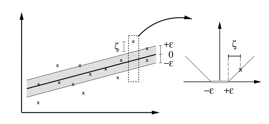
Figure by Smola and Schölkopf (2003): A Tutorial on Support Vector Regression

Like Support Vector Classification (Session 5), SVR can deploy the kernel trick, which allows for solving non-linear problems within a higher dimensional feature data space, making it a very flexible regression method.

Synthetic training data

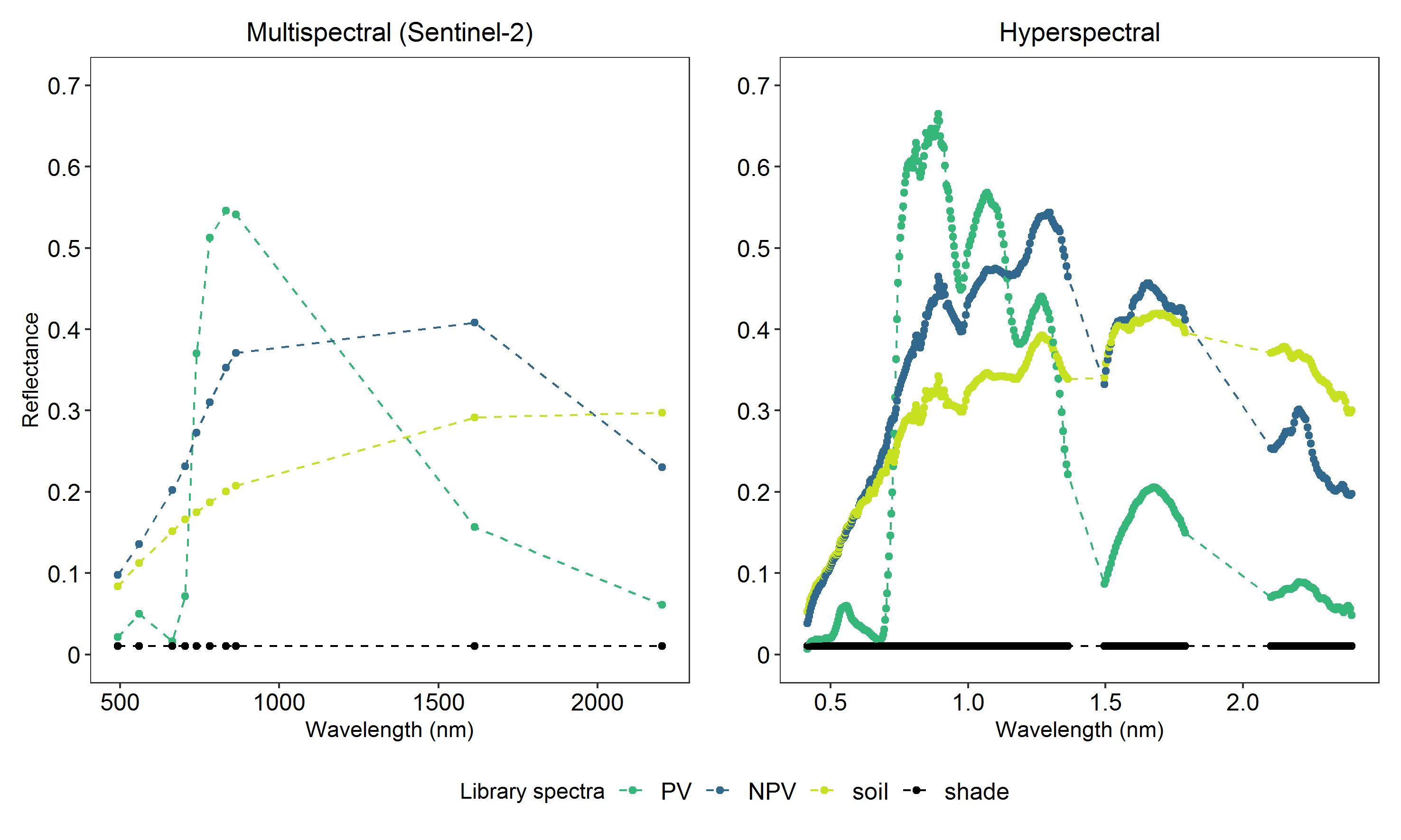
We need representative data to train the regression models. Obtaining representative continuous training data for several cover types is often expensive and sometimes not feasible at all for the time and area of interest. Therefore, instead of using e.g. training data collected in the field, we can create synthetic training data. Based on the assumption for linear spectral unmixing, we know that the proportion of the spectral signature of a certain class in a mixed pixel corresponds to its cover fraction on the ground. We can therefore create the spectral signature of any cover fraction between 0 and 100% using the pure (i.e. 100%) spectral signature of the class. These pure spectra are often called “endmembers”. Endmembers can be spectral measurements collected in the field or the laboratory, then compiled in a spectral library (e.g. the USGS HRSL, or they can be extracted from the satellite data directly (image endmembers).

These are examples of spectral libraries from multispectral and hyperspectral images for photosynthetic vegetation (PV), non-photosynthetic vegetation (NPV), soil and shade:

By assigning weights between 0 and 1 (i.e. 0-100% cover) and combining the weighted pure spectra linearly, training samples for the regression models can be generated:

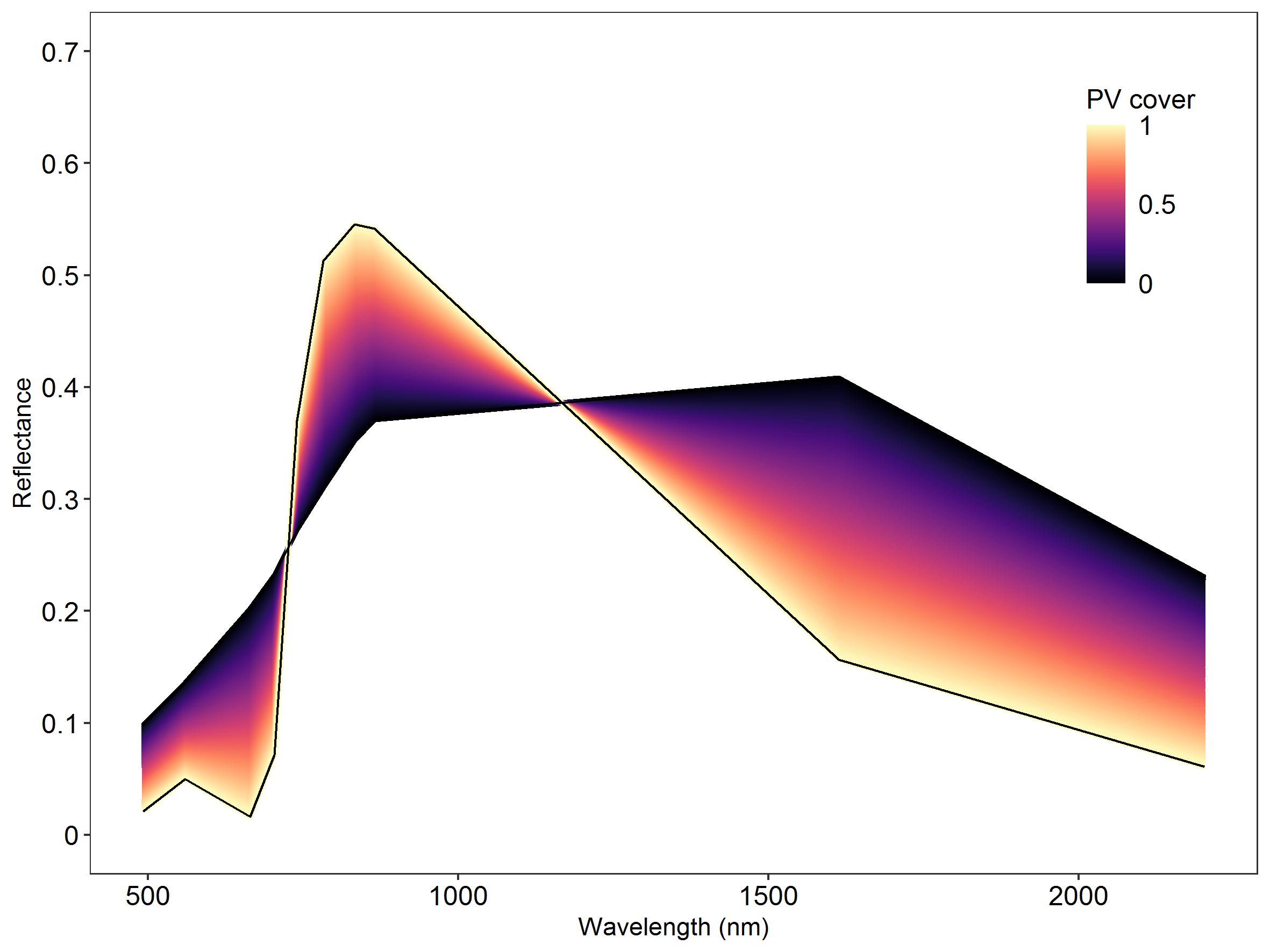
Linear mixtures of the two Sentinel-2 library spectra PV (target class) and NPV with randomly assigned weights under the constraint of summing to 1.

Evaluation of quantitative model predictions

To evaluate the results of the regression model, we need independent validation data. There a variety of sources and methods to obtain validation data for fractional cover. Some examples are:

field data collection (e.g. point sampling)
visual analysis of high resolution data (e.g. Google Earth)
image segmentation of, e.g., datasets from Unmanned Aerial Vehicles (UAV)
regression-based unmixing of datasets with sufficient spatial and spectral resolution (e.g. hyperspectral images)

For model evaluation, it is often helpful to plot the observed and predicted values in form of a scatterplot. Ideally, we expect a perfect linear relation of observed and predicted values. Therefore, assessing the results of a linear regression of the predicted and observed values provides the information for evaluating the agreement of the observed and predicted data.

Several measures of agreement can be calculated from predicted and observed data:

Regression slope and intercept

\[ y_i = ß_0 + ß_1\hat{y_i} + \epsilon \] where $y_i$ is the observed value, $\hat{y_i}$ is the predicted value, $ß_0$ is the intercept, $ß_1$ is the slope and $\epsilon$ is the random error term.

for the slope, $ß_1$, a value close to 1 indicates that observed and predicted values vary consistently within their range
the intercept, $ß_0$, can only be interpreted as the bias when the slope is 1.

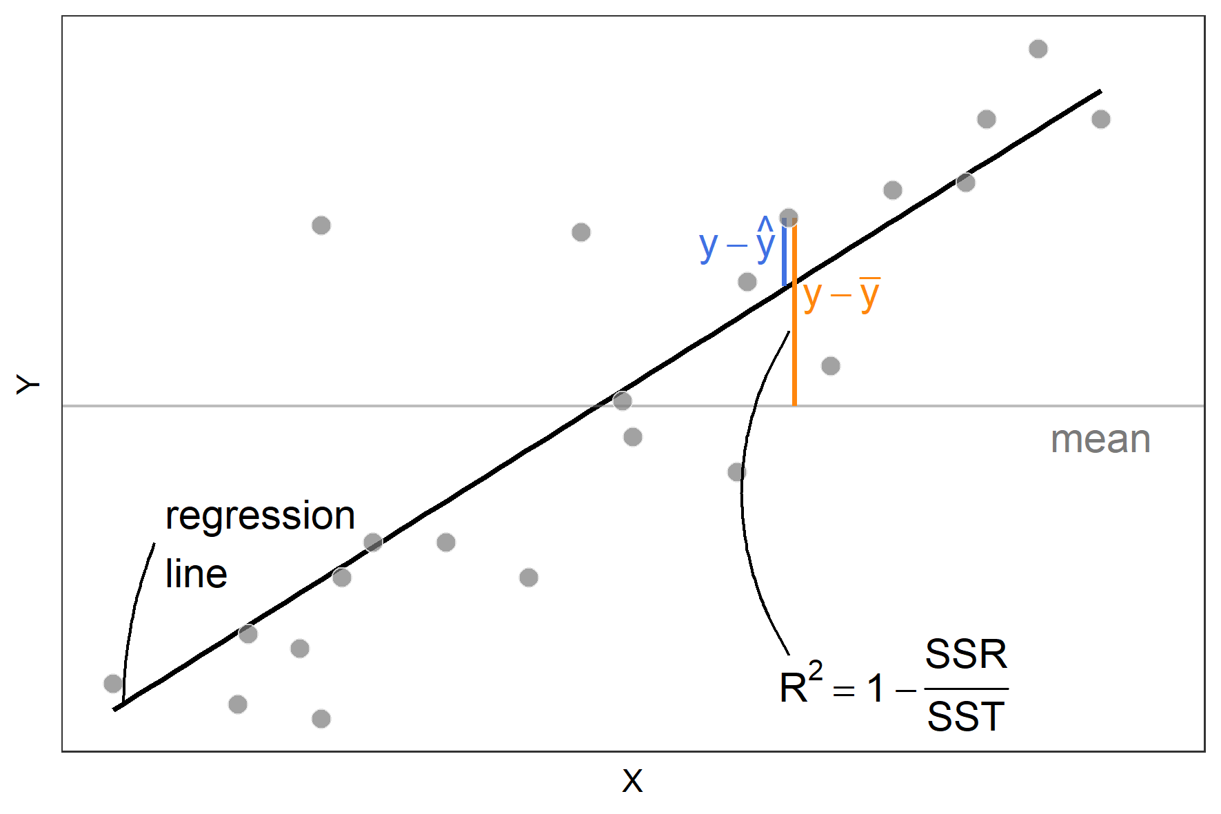
Coefficient of determination

describes the percentage of the variance in the observed values explained by the variance of the predicted values
$R^2$ is also the square of the Pearson correlation coefficient R in the case of simple linear regression with one predictor. $R^2$ is easier to interpret than Pearsons correlation coefficient, e.g., $R^2 = 0.8$ explains twice as much variance as $R^2=0.4$

\[ R^2 = 1- \frac{ \sum_{i=1}^n (y_i- \hat{y_i})^2}{\sum_{i=1}^n (y_i - \overline{y_i})^2} \] where $y_i$ is the observed value, $\hat{y_i}$ is the predicted value and $\overline{y}$ is the mean of the observed values. The numerator in this formula is the sum of squares residual (SSR) and the denominator is the sum of squares total (SST):

Mean Absolute Error

describes the average error of the predicted values without considering the error direction
modeling unit is preserved

\[ MAE = \frac{1}n \sum_{i=1}^n |y_i - \hat{y_i}| \]

Root Mean Square Error

is the mean deviation of predicted values with respect to the observed values
modeling unit is preserved
by squaring the error, RMSE penalizes higher deviations stronger than the MAE i.e. it is always higher than (in rare cases equal to) the MAE

\[ RMSE = \sqrt{\frac{1}n \sum_{i=1}^n(y_i - \hat{y}_i)^2}\]

Prediction bias

is the systematic error of the predicted values with regards to the observed data

\[ Bias = \frac{1}n \sum_{i=1}^n y_i - \frac{1}n \sum_{i=1}^n \hat{y_i}\]

Note: When creating a scatterplot of observed and predicted data and evaluating the linear regression function, the observed values correspond to the y-axis and the predicted values to the x-axis. Interchanging these positions will lead to incorrect slope and intercept values.

Assignment

In this assignment, you will learn how you can use SynthMix and Support Vector Regression to obtain fractional vegetation and soil cover for crop and grassland fields in northeastern Germany from 10m Sentinel-2 data. You will also learn how to quantitatively evaluate your fractional cover estimates with a reference dataset.

Here you can download the data needed for completing the assignment.

The zip-file contains these files:

Sentinel-2 image, BOA reflectance, cloud-masked, date of acquisition: 26.07.2019
Spectral library with pure spectra of PV, NPV and soil from the Sentinel-2 image
Validation points (.gpkg) for the date of image acquisition to evaluate predictive performance

Please install and load the packages needed for this assignment. We use three packages from the tidyverse (ggplot2, tidyr and dplyr). These packages are very useful for handling and manipulating your data in R. If you are interested, you can find a very short overview of the capabilities of the tidyverse packages here.

pck_list <- c("assertthat","ggplot2", "tidyr", "dplyr","raster", "e1071", "rgdal", "viridisLite")
lapply(pck_list, require, character.only = TRUE)

1) Input spectra

Let’s first take a look at our input data: the pure endmember spectra which represent 100% surface cover of our four classes. We consider these spectra as representative of the three target classes of PV, NPV, and soil and add a shade spectrum to account for variation in brightness caused by, e.g. high vegetation.

Load the spectral library containing the three class spectra of PV, NPV and soil into R (S2_EM.txt). The BOA reflectance of the endmembers was scaled by 10,000.

Visualize the spectral signatures of PV, NPV, soil and shade as line plot using ggplot2. For a better visualization, use the central wavelengths of the Sentinel-2 bands (find them here) and add them to your data.frame.
What are the main characteristics of the spectra? How do the spectra differ between the classes and which wavelength regions could be most important for differentiating the classes?

2) Linear spectral mixtures

Based on the pure endmembers, we now want to simulate a “mixed pixel”. We can do this be defining the desired cover proportions of the different surface components, e.g.:

fraction_PV <- 0.1      # 10% PV
fraction_NPV <- 0.8     # 80% NPV
fraction_soil <- 0.05   # 5% Soil
fraction_shade <- 0.05  # 5% shade

# Do we violate the assumption that all surface components represent 100% of the surface area?
if((fraction_PV + fraction_NPV + fraction_soil+ fraction_shade) != 1) print('Fractions don´t sum to 1.')

Next we can create a (synthetic) linear mixture of the endmember spectra by weighting each pure spectra using the defined cover proportions from above. In the previous task, we had already read in the endmember file and called it slib:

# Create a linear mixture of the endmember spectra
model_spectrum <- fraction_PV * slib$PV + 
                  fraction_NPV * slib$NPV +
                  fraction_soil * slib$soil + 
                  fraction_shade * slib$shade

# We could simulate imperfect measurements by adding random noise.
noise <- rnorm(10, mean=0, sd=0.02)

# Append the modeled spectrum to the endmembers data.frame
slib$model_spectrum <- model_spectrum + noise

# Convert the spectra into long format for plotting with ggplot2
slib_vis <- pivot_longer(slib, -c(band, cwl)) 

# Visualize the modeled spectrum in comparison to the endmember spectra
ggplot(sli_vis) + 
  geom_line(aes(x=cwl, y=value, color=name, linetype=name))+
  scale_color_manual(values=c("black", "steelblue", "darkgreen", "darkgrey","firebrick"), name="Spectrum")+
  scale_linetype_manual(values=c("dotdash", rep("solid", 4)), name="Spectrum")+
  scale_y_continuous(labels=seq(0,1,0.1), breaks=seq(0,10000,1000))+
  theme_bw()+
  theme(panel.grid=element_blank())+
  labs(x="Wavelength (nm)", y="Reflectance")

3) Synthetic training data generation

Now that we know the principles and practical steps of synthetic linear mixing, we can use the function below to generate synthetic training data for a large variety of mixture combinations. Here, we will stick to our four endmembers (one for each class), but note that we can in theory (and usually do) use a large variety of different endmember spectra for each of the classes.

Why can it be beneficial to use not only one, but many endmember spectra for each class?

Now take a look at the synthmix function which provides you with a variety of settings for creating your artificial mixtures. Read the function description to understand what each argument represents and what type of user input it expects:

synthmix <- function(df, cl_target, cl_background, n_samples=1000,
                     mix_complexity=c(2, 3, 4), p_mix_complexity=c(.7, .2, .1),
                     within_class_mixture=TRUE, include_endmember=TRUE){
  
  "Function to generate synthetic training data mixtures from pure endmember
  spectra.
  
  df:                 (list) Input dataframe. First column must contain the
                      class-IDs in integer format. Remaining columns must 
                      contain the features to be mixed. 
  cl_target:          (int) Target class' integer ID value.
  cl_background:      (int) Background class' integer ID value(s). Vector for 
                      multiple classes, e.g. 'c(2, 3, 4)'.
  n_samples:          (int) Number of synthetic training points to generate.
  mix_complexity:     (int) Vector with desired number of possible mixtures
                      between different classes.
  p_mix_complexity:   (float) Vector containing desired occurence propabilities 
                      associated to the number of possible mixtures 
                      (i.e. mix_complexity). Must be of same length as 
                      'mix_complexity' argument.
  
  returns:            (list) Dataframe with linearily mixed features and 
                      corresponding fraction of target class (i.e. cl_target)
  "
  
  # total number of classes
  all_ems <- c(cl_target, cl_background)
  n_em <- length(all_ems)
  
  # create empty df to store training data
  df_mixture <- setNames(data.frame(matrix(ncol = ncol(df), nrow = 0)), 
                          c(names(df)[2:length(df)], "fraction")) 
  
  # index list of EMs for sampling
  idx_em <- list()
  for (em in all_ems){
    idx_em[[em]] <- which(df[,1] == em)
  }
  
  # vector for fraction calculation
  zero_one <- integer(nrow(df))
  zero_one[idx_em[[cl_target]]] <- 1
  
  # iterator for generating each synthetic mixture 
  for (i in 1:n_samples) {
    
    if (length(p_mix_complexity) == 1){
      complexity = mix_complexity
    } else {
      # sample mixing complexity based on mixing likelihoods
      complexity = sample(as.vector(mix_complexity), 
                    size = 1, 
                    prob = as.vector(p_mix_complexity)) 
    }
    
    # select background EMs which will be included in the mixture
    if (within_class_mixture){
      background <- sample(all_ems, complexity - 1, replace = TRUE)
    } else {
      background <- sample(cl_background, complexity - 1, replace = FALSE)
    }
    
    # sample indices of selected EMs
    response <- c(cl_target, background)      
    drawn_index <- c()
    for (r in response){
      drawn_index <- c(drawn_index, sample(idx_em[[r]], 1))
    }
    drawn_features <- df[drawn_index, 2:length(df)]
    drawn_fraction <- zero_one[drawn_index]
    
    # sample random weights
    drawn_weights <- c()
    for (j in 1:(complexity-1)){
      if (j == 1){
        weight <- runif(1)
      } else {
        weight <- runif(1) * (1. - sum(drawn_weights))
      }
      drawn_weights <- c(drawn_weights, weight)
    }
    drawn_weights <- c(drawn_weights, (1. - sum(drawn_weights)))
    
    # calculate mixtures and associated fractions
    calc_mixtures <- apply(drawn_features * drawn_weights, 2, FUN=sum)
    calc_fraction <- sum(drawn_fraction * drawn_weights)
    
    # append to df
    df_mixture[nrow(df_mixture)+1,] <- c(calc_mixtures, calc_fraction)
  }
  
  if (include_endmember){
    df_endmember <- cbind(df[,2:length(df)], zero_one)
    colnames(df_endmember) <- c(names(df)[2:length(df)], "fraction")
    df_mixture <- rbind(df_mixture, df_endmember)
  }
  
  return(df_mixture)

}

Now the first argument is the input data.frame containing our pure endmember spectra. Note that the function expects the data to be arranged in a specific way: “First column must contain the class-IDs in integer format. Remaining columns must contain the features to be mixed”.

Format your data.frame to meet the function’s criteria.

When the input data is prepared and the function is understood:

Use the synthmix function to create an individual (class-wise) data.frame with 1,000 linear mixtures for each of the three main target classes (PV, NPV, soil). Use a 50/50 probability of 2- and 3-endmember mixtures. The pure library spectra are added automatically to the final set of spectra.

4) Modeling fractional cover

Having the training data in place, we want to train a Support Vector Regression (SVR) and a Random Forest Regression (RFR) model for the first target class using the synthetic training data. Try the svm() function from the e1071 package for SVR modeling and the randomForest from the previous session for RFR. The functions infer the model type (regression vs. classification) from the type of the data (although you can be explicit for RFR by setting type= “regression”) and set several default parameters. Contrary to RFR, SVR is very sensitive to parameterization - which means to get good results, it is necessary to tune the model by trying different parameter combinations. Use the tune.svm() function to perform a grid search with 10-fold cross validation for the parameters cost and gamma. It is advised to vary the parameters between 10^-3 and 10^3 with logarithmic steps (i.e. 0.001, 0.01, 0.1 etc.). The best parameter set is internally determined by the function using the mean squared error (MSE). Set the epsilon parameter to 0.001.

For each class (PV, NPV, Soil), build (and tune) a RFR and SVR model. For SVR, extract the best model from the resulting object with $best.model.
Use predict() to estimate the fractional cover of each class for the Sentinel-2 image. The model will expect predictors named identical to the input data you used for training (i.e. ‘Bxx’). Rename the bands of the Sentinel-2 image (here s2) with names(s2) <- paste("B", seq(1,10), sep="").
Stack and export the fractional cover predictions for each model with writeRaster.
Visualize the fractional cover as RGB color combination (e.g. soil, PV, NPV) in QGIS. Remember to set the stretch from 0-1. Based on this, can you identify fields in different stages of the crop phenology?

5) Evaluation of fractional cover

Last, we want to evaluate the model predictions based on independent validation data. The file validation_20190726.gpkg contains the validation points and the corresponding fractional cover values. The values of the validation data range between 0 and 1.

Load the vector file into R and extract the values of the fraction cover predictions.
Set negative values of the predicted values to 0 and super-positive values (i.e. > 1) to 1.
Create a scatterplot of predicted and observed fractional cover values for each class (and algorithm).
Calculate $R^2$, $MAE$, $RMSE$ and slope and intercept of the simple linear regression and add them to your plot. How do they differ between PV, NPV and soil? How do SVR and RFR compare?

# You can use this function to calculate the simple linear regression coefficients 
# of observed and predicted data and annotate it in your plots
lm_eqn <- function(pred_x,obs_y,df){
  m <- lm(obs_y ~ pred_x, df);
  eq <- substitute(y ==  a + b * x,
                   list(a = format(as.numeric(round(coef(m)[1]/100,2))),
                        b = format(as.numeric(round(coef(m)[2],2)))))
  as.character(as.expression(eq));
}

# For a better visualization, you can use this function to calculate the point
# density and display it as the color in your scatterplots:
get_density <- function(x, y,...) { # set x and y to predicted and observed values and n = 100
  dens <- MASS::kde2d(x, y, ...)
  ix <- findInterval(x, dens$x)
  iy <- findInterval(y, dens$y)
  ii <- cbind(ix, iy)
  return(dens$z[ii])
}