Recap GLMs

Generalization of linear models that allow to choose freely

how the data is linked to the model (link-function) and
which data generating distribution is assumed (data distribution).

We covered four models:

Log link and Gaussian distribution for bounded numerical response data (ozone~temp)
Logit link and binomial distribution for proportional response data (mortality~concentration)
Logit link and binomial distribution for binary response data (infestation~temp_anomaly)
Log link and Poisson distribution for count response data (bird_count~topo_relief)

In R, GLMs are constructed using the glm() function.

Today’s session

Distribution functions in R
Model checking using simulations

Packages

require(ggplot2)
require(tidyverse)
require(effects)

Distributions in R

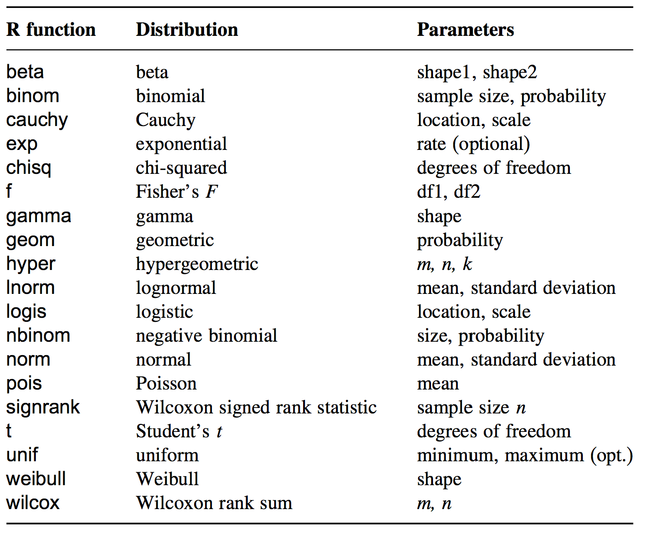
Four fundamental items can be calculated for a statistical distribution:

Density or point probability (abbreviated by d)
Cumulated probability, distribution function (abbreviated by p)
Quantiles (abbreviated by q)
Pseudo-random numbers (abbreviated by r)

For all distributions implemented in R, there is a function for each of the four items listed above. For example, for the normal distribution, these are named dnorm, pnorm, qnorm, and rnorm.

Probability distribution function

x <- seq(-4, 4, length = 100)

normal_dist <- data.frame(x = x,
                          d1 = dnorm(x = x, mean = 0, sd = 1),
                          d2 = dnorm(x = x, mean = 0.5, sd = 2),
                          d3 = dnorm(x = x, mean = -1, sd = 0.5))

ggplot(normal_dist) +
  geom_line(aes(x = x, y = d1), col = "blue") +
  geom_line(aes(x = x, y = d2), col = "red") +
  geom_line(aes(x = x, y = d3), col = "green") +
  labs(x = "x", y = "N(x)")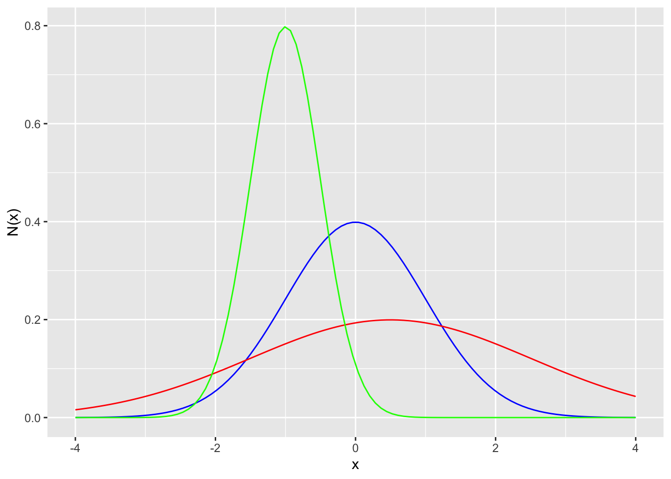

Cummulative distribution function

normal_dist <- normal_dist %>%
  mutate(p1 = pnorm(q = x, mean = 0, sd = 1),
         p2 = pnorm(q = x, mean = 0.5, sd = 2),
         p3 = pnorm(q = x, mean = -1, sd = 0.5))

ggplot(normal_dist) +
  geom_line(aes(x = x, y = p1), col = "blue") +
  geom_line(aes(x = x, y = p2), col = "red") +
  geom_line(aes(x = x, y = p3), col = "green") +
  labs(x = "x", y = "Cummulative N(x)")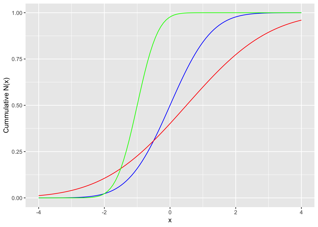

Inverse cummulative distribution function

z_95 <- qnorm(p = 0.95, mean = 0, sd = 1)

ggplot(normal_dist) +
  geom_line(aes(x = x, y = p1), col = "blue") +
  geom_vline(xintercept = z_95) +
  labs(x = "x", y = "density")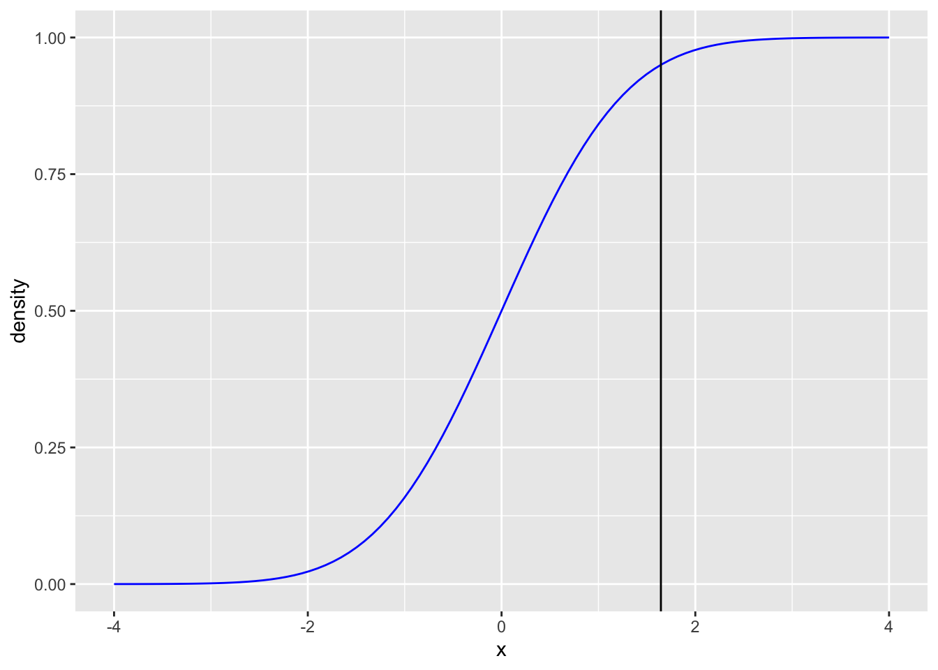

Random draws

random_normal <- data.frame(r1 = rnorm(n = 100, mean = 0, sd = 1),
                            r2 = rnorm(n = 100, mean = 0, sd = 1))

ggplot(random_normal, aes(x = r1, y = r2)) +
  geom_point() +
  labs(x = "random draws", y = "random draws")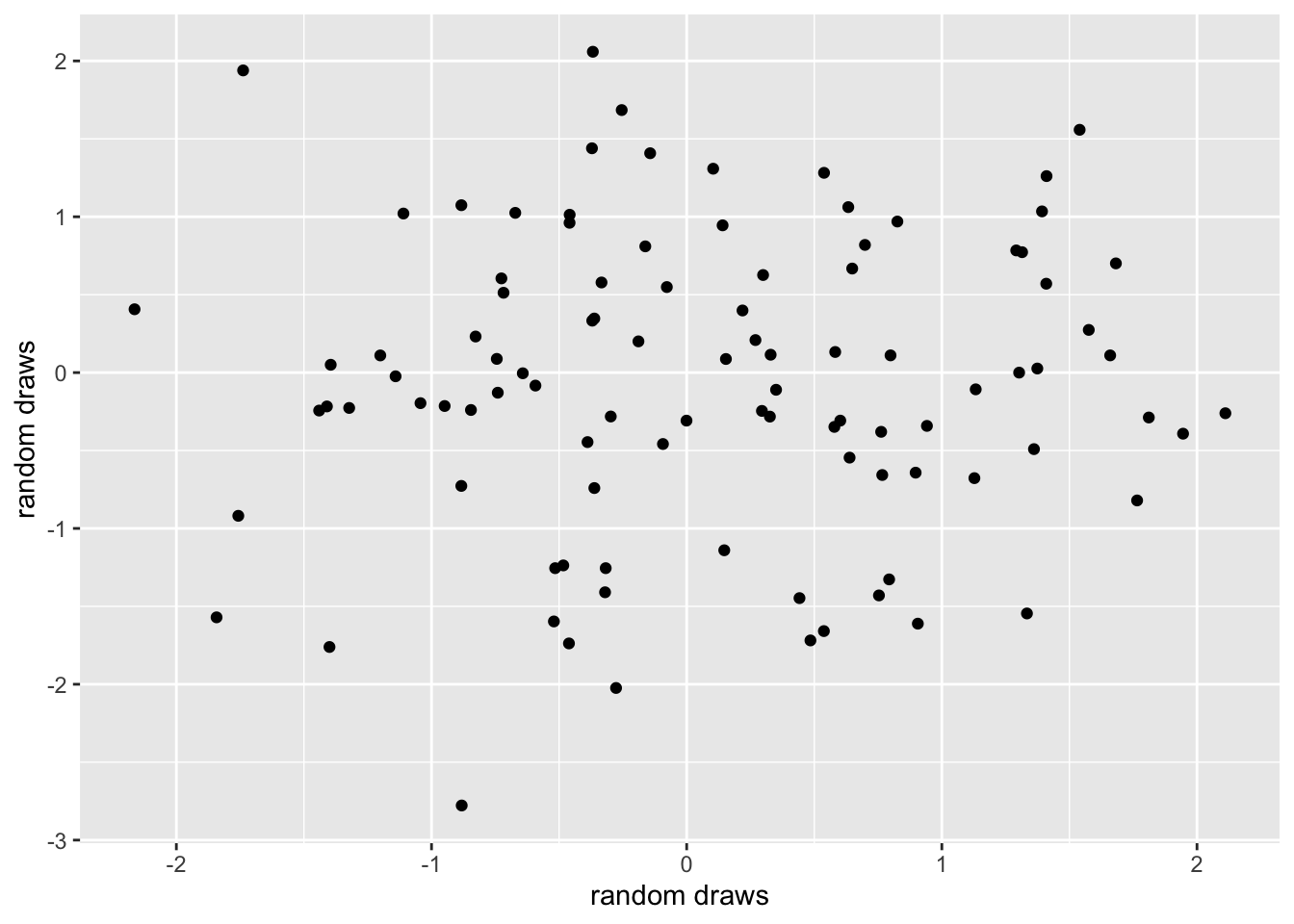

Simulations

Estimate uncertainty in regression coefficients
Construct the predictive interval
Check statistical procedures

Simulating uncertainty in regression coefficients

Simulation can be useful to summarize uncertainty estimates for multiple parameters

library(arm)
heights <- read.csv ("Data/heights.csv")
ht.lm <- lm(log.earn ~ height+male+height:male, data=heights)
summary(ht.lm)

## 
## Call:
## lm(formula = log.earn ~ height + male + height:male, data = heights)
## 
## Residuals:
##     Min      1Q  Median      3Q     Max 
## -4.2375 -0.3380  0.1504  0.5674  2.2595 
## 
## Coefficients:
##              Estimate Std. Error t value Pr(>|t|)    
## (Intercept)  8.693956   0.934868   9.300   <2e-16 ***
## height       0.012565   0.014432   0.871    0.384    
## male        -0.122068   1.365947  -0.089    0.929    
## height:male  0.008396   0.020232   0.415    0.678    
## ---
## Signif. codes:  0 '***' 0.001 '**' 0.01 '*' 0.05 '.' 0.1 ' ' 1
## 
## Residual standard error: 0.8938 on 1055 degrees of freedom
## Multiple R-squared:  0.08348,    Adjusted R-squared:  0.08088 
## F-statistic: 32.03 on 3 and 1055 DF,  p-value: < 2.2e-16

For classical linear regression and generalized linear models, a simulation function sim() is implemented in the arm package.

n.sims <- 1000
ht.sim <- sim(ht.lm, n.sims)
head(ht.sim@coef)

##      (Intercept)       height      male   height:male
## [1,]    9.613395 -0.002101922 -0.844546  0.0205495306
## [2,]    8.825312  0.009943661 -1.061259  0.0214333255
## [3,]   10.071711 -0.009668765 -1.099175  0.0245016205
## [4,]    9.374188  0.001912586 -1.198182  0.0241636125
## [5,]    8.642715  0.013673797  0.493189 -0.0002885298
## [6,]    8.136169  0.021456532  0.770125 -0.0060998501

Gelman and Hill (2007). Data Analysis Using Regression and Multilevel/Hierarchical Models

hist(ht.sim@coef[,2])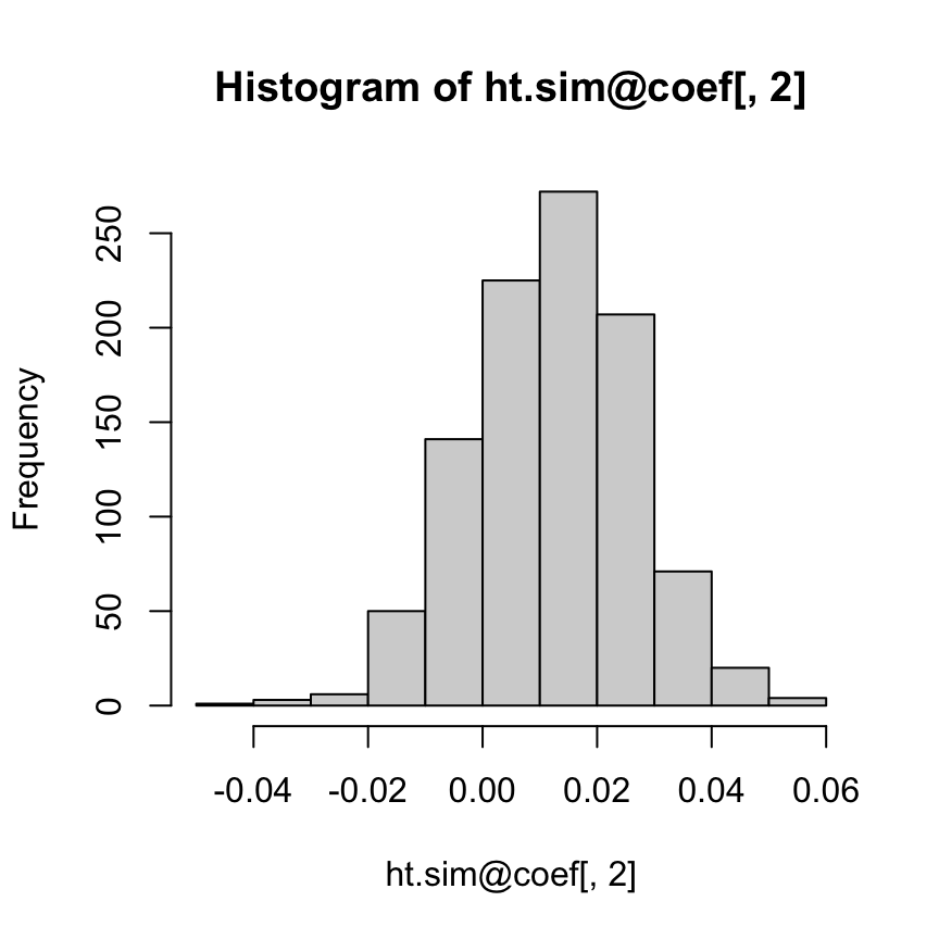

In this interaction model, what can be said about the coefficient of height among men? We cannot directly answer this question using the regression output: the slope for men is a sum of the height and height:male coefficients, and there is no simple way to compute its standard error given the information in the regression table. The most direct approach is to compute the 95% interval directly from the inferential simulations:

height.for.men.coef <- ht.sim@coef[,2] + ht.sim@coef[,4]
quantile(height.for.men.coef, c(0.025, 0.975))

##         2.5%        97.5% 
## -0.005530046  0.049505173

Statistical significance is not the object of the analysis - but it is important to have a sense of the uncertainty of estimates.

Simulating OLS

We assume that the outcome we are interested in studying follows some probability distribution that has one or more unknown parameters that we need to estimate. In OLS, the response variable (\(Y\)) is a function of an intercept \(\beta_0\), coefficients for explanatory variables (\(\beta\) and \(X\), respectively), and an error term that is assumed to follow a normal distribution (\(\epsilon\)).

\[Y = \beta_0 + \beta_1X_1 + \beta_2X_2 +... + \epsilon\]

\[\epsilon \sim \mathcal{N}(0, \sigma)\]

Another way to describe this model is to write \(Y\) as following a normal distribution, and the explanatory variables inform estimates of \(\mu\) and/or \(\sigma\). In this representation, Y is normally distributed with mean (\(\mu\)) and a constant standard deviation (\(\sigma\)). The second line of the model expresses \(\mu\) as the fitted linear equation. In other words, the response variable is explicitly written as following a probability distribution with its mean set to a linear combination of coefficients and explanatory variables.

\[Y \sim \mathcal{N}(\mu, \sigma)\]

\[\mu = \beta_0 + \beta_1X\]

\[Y \sim \mathcal{N}(\beta_0 + \beta_1X, \sigma)\]

Let’s simmulate a linear response by setting the parameters of the above equation (supposedly) known values. To simulate the response we will draw from a normal distribution \(n=1000\) samples.

n <- 1000 # sample size

b0 <- 0.2 # true value for the intercept
b1 <- 0.5 # true value for the slope
sigma <- 0.2

# create sample of n observations for independent variable X
# X is set to range from -1 to 1
X <- runif(n, -1, 1) 

# We can simulate the true response by adding a random error term (epsilon)
Y <- b0 + b1*X + rnorm(n, 0, sigma)

# But we can also write the above equation as follows
Y <- rnorm(n, b0 + b1*X, sigma)

plot(X, Y, pch=16, col=rgb(0,0,0,0.3))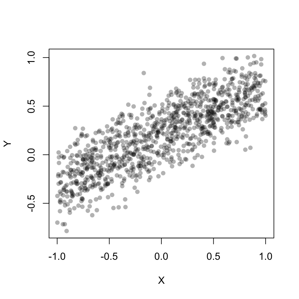

Now, lets fit a linear model throught the simulated Y. You should recognize the estimated coefficients (our \(\beta's\)). The residual standard error (actually residual standard deviation) is our \(\sigma\).

lmd <- lm(Y ~ X)
summary(lmd)

## 
## Call:
## lm(formula = Y ~ X)
## 
## Residuals:
##      Min       1Q   Median       3Q      Max 
## -0.56864 -0.14754  0.00175  0.14509  0.72264 
## 
## Coefficients:
##             Estimate Std. Error t value Pr(>|t|)    
## (Intercept) 0.203103   0.006455   31.47   <2e-16 ***
## X           0.501953   0.011614   43.22   <2e-16 ***
## ---
## Signif. codes:  0 '***' 0.001 '**' 0.01 '*' 0.05 '.' 0.1 ' ' 1
## 
## Residual standard error: 0.2041 on 998 degrees of freedom
## Multiple R-squared:  0.6518, Adjusted R-squared:  0.6514 
## F-statistic:  1868 on 1 and 998 DF,  p-value: < 2.2e-16

Confidence and prediction interval

Setting the argument interval = "confidence" you get the vector of predicted values with a lower and upper limit given uncertainty in the parameters.
If you add interval = "prediction", then you get the vector of predicted values with a lower and upper limit given uncertainty in the parameters plus residual variance.
Note, R by default returns the 95% confidence interval. You can change it by seting the argument level to another confidence level (e.g., level = 0.99).

df <- data.frame(X=X, Y=Y, predict(lmd, interval = 'confidence'))
names(df)[4:5] <- c('conf_lwr', 'conf_upr') 
df <- cbind(df, predict(lmd, interval = 'prediction')[,2:3])

## Warning in predict.lm(lmd, interval = "prediction"): predictions on current data refer to _future_ responses

names(df)[6:7] <- c('pred_lwr', 'pred_upr') 

ggplot(df, aes(x = X, y = Y)) +
  geom_point(col='gray')+
  geom_line(aes(y=fit), col='black') +
  geom_ribbon(aes(ymin=pred_lwr, ymax=pred_upr, fill="Prediction band"), alpha = 0.3) +
  geom_ribbon(aes(ymin=conf_lwr, ymax=conf_upr, fill="Confidence band"), alpha = 0.6)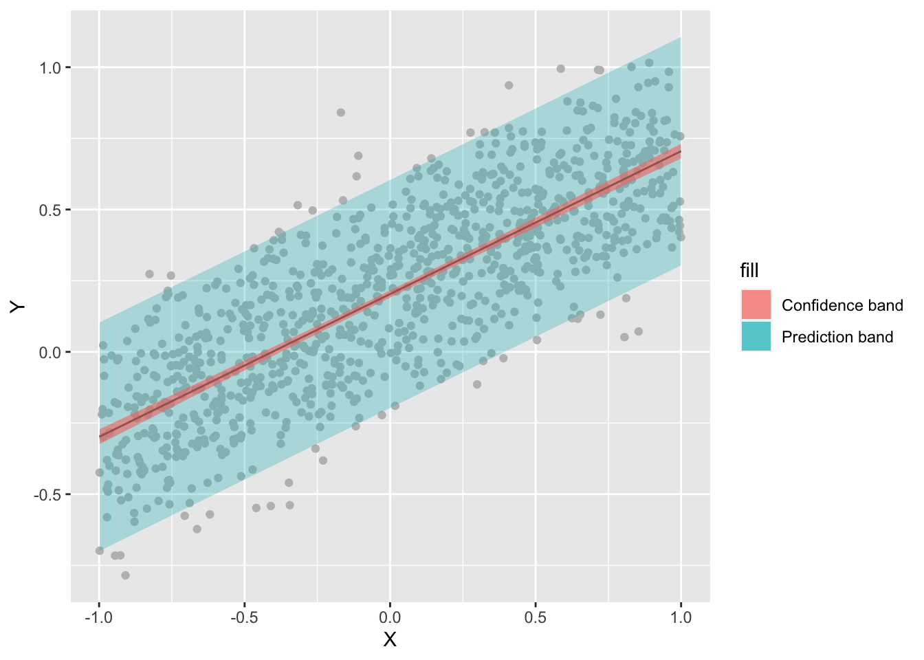

Logistic regression

Now we will simulate a logistic regression model. The logit model is written as follows:

\[logit(Pr(Y=1)) = \mu\] \[ Pr(Y=1) = logit^{-1}(\mu)\] \[\mu = \beta_0 + \beta_1X\]

We use the inverse logit function (\(logit^{-1}\)) to calculate the probability of observing \(Y=1\). Recall, the inverse logit function in R is plogis().

n <- 1000 # sample size

b0 <- 1 # true value for the intercept
b1 <- 10 # true value for the slope

# create sample of n observations for independent variable X
# X ranges from -1 to 1
X <- runif(n, -1, 1) 

# We use rbinom to make random draws from a binomial distribution
Y <- rbinom(n, 1, plogis(b0 + b1*X))

glmd <- glm(Y ~ X, family=binomial(link='logit'))
summary(glmd)

## 
## Call:
## glm(formula = Y ~ X, family = binomial(link = "logit"))
## 
## Deviance Residuals: 
##     Min       1Q   Median       3Q      Max  
## -3.3346  -0.1594   0.0181   0.1602   2.9308  
## 
## Coefficients:
##             Estimate Std. Error z value Pr(>|z|)    
## (Intercept)   0.7794     0.1429   5.453 4.97e-08 ***
## X             8.9093     0.6539  13.624  < 2e-16 ***
## ---
## Signif. codes:  0 '***' 0.001 '**' 0.01 '*' 0.05 '.' 0.1 ' ' 1
## 
## (Dispersion parameter for binomial family taken to be 1)
## 
##     Null deviance: 1375.46  on 999  degrees of freedom
## Residual deviance:  379.39  on 998  degrees of freedom
## AIC: 383.39
## 
## Number of Fisher Scoring iterations: 7

ds.sim <- data.frame(X=X, Y_sim=Y, Y_fit=fitted(glmd))
ggplot() +
  geom_point(data = ds.sim, aes(x = X, y = Y_sim), alpha = 0.1, col = "red") +
  geom_line(data = ds.sim, aes(x = X, y = Y_fit))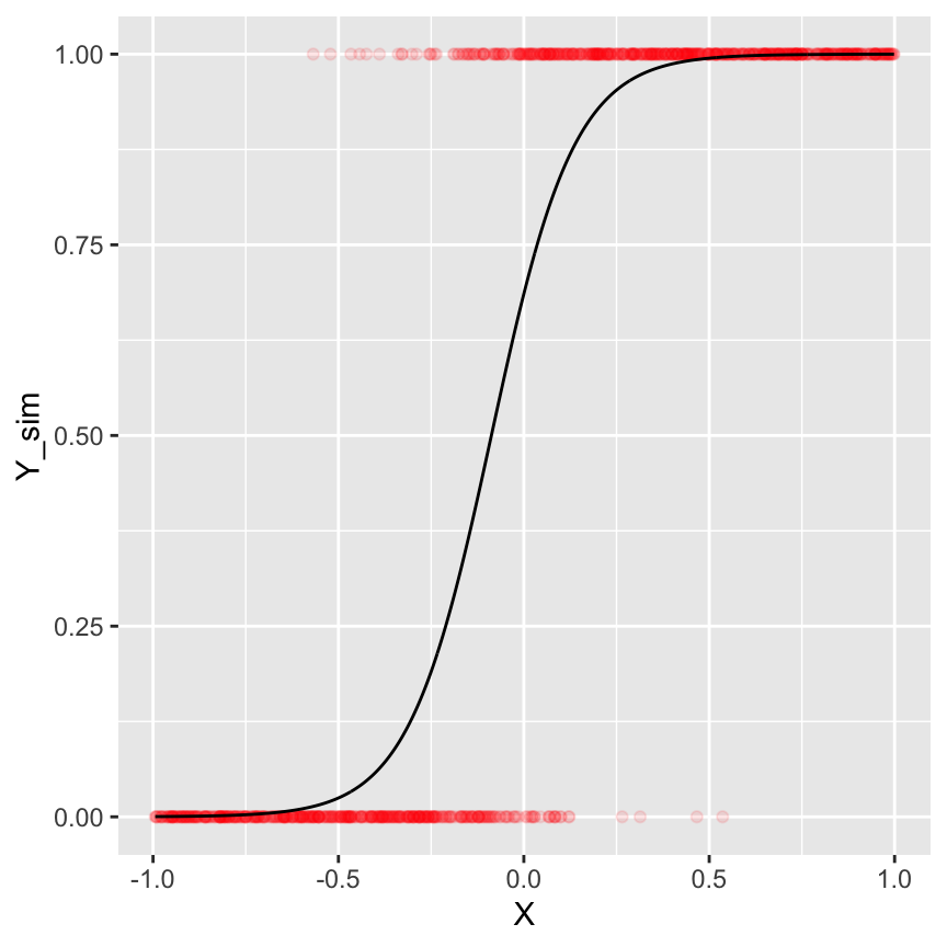

Poisson regression (Counts)

Recall, the Poisson distribution has one parameter \(\lambda\), which is both the mean and variance of the distribution. Poisson regression links the systematic portion of the model to a Poisson distribution through \(\lambda\). It assumes the natural log of the dependent variable’s expected value can be modeled by a linear combination of explanatory variables.

\[log(E(Y)) = \mu\] \[E(Y) = exp(\mu)\] \[\mu = \beta_0 + \beta_1X\]

Now, we fit a Poisson regression model to the bird count data. Then, we simulate bird counts (response) using the estimated parameters. Finally, we compare the simulated bird counts with the observed bird counts to understand whether our Poisson model behaves as we would expect from the real observations.

dat <- read.table("Data/bird_counts.txt", sep = ";", header = TRUE)

glmd <- glm(Y ~ relief, data=dat, family=poisson(link = "log"))

dat$Y_fit <- fitted(glmd)

summary(glmd)

## 
## Call:
## glm(formula = Y ~ relief, family = poisson(link = "log"), data = dat)
## 
## Deviance Residuals: 
##      Min        1Q    Median        3Q       Max  
## -11.1980   -2.1407   -0.0021    2.1986   10.7204  
## 
## Coefficients:
##             Estimate Std. Error z value Pr(>|z|)    
## (Intercept) 4.665888   0.021577  216.24   <2e-16 ***
## relief      0.339559   0.008382   40.51   <2e-16 ***
## ---
## Signif. codes:  0 '***' 0.001 '**' 0.01 '*' 0.05 '.' 0.1 ' ' 1
## 
## (Dispersion parameter for poisson family taken to be 1)
## 
##     Null deviance: 2921.1  on 60  degrees of freedom
## Residual deviance: 1299.6  on 59  degrees of freedom
## AIC: 1739.7
## 
## Number of Fisher Scoring iterations: 4

b0 <- coef(glmd)[1]
b1 <- coef(glmd)[2]
n <- 10000

# create sample of n observations for independent variable X
X <- runif(n, min=min(dat$relief), max=max(dat$relief))

# Use rpois to make random draws from a poisson distribution
Y <- rpois(n, lambda=exp(b0 + b1*X))

ds.sim <- data.frame(relief=X, Y_sim=Y)
ggplot() +
      geom_point(data = ds.sim, aes(x = relief, y = Y_sim), alpha = 0.1, col = "red") +
      geom_point(data = dat, aes(x = relief, y = Y)) +
      geom_line(data = dat, aes(x = relief, y = Y_fit))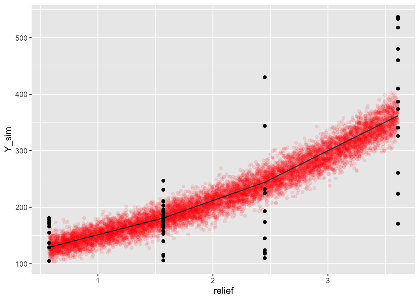

Tackling overdispersion

Our model shows signs of overdispersion. Overdispersion means that the data shows greater variability than would be expected based on our model.

Overdispersion is pretty common with poisson regression as the poisson distribution does not have a variance term that is estimated from the data, but \(var = \mu\).

We can overcome the problem of overdispersion by using a quasipoisson data distribution, which assumes that the variance increases with the mean via a pre-defined function such as \(var = c*\mu\).

The problem with quasipoisson, however, is that it uses quasi-likelihoods which prevents use from calculating several useful things such as the AIC.

Alternatively, we can specify a negative binomial model, which has a dispersion parameter \(\theta\):

\(counts \sim NegBinom(log^{-1}(\beta_0 + \beta_1 * relief), \theta)\)

Negative binomial GLM

Fitting a negative binomial model in R using the glm.nb() function in the MASS package:

library(MASS)

fit <- glm.nb(Y ~ relief, data = dat, link = "log")

## 
## Call:
## glm.nb(formula = Y ~ relief, data = dat, link = "log", init.theta = 11.71533906)
## 
## Deviance Residuals: 
##      Min        1Q    Median        3Q       Max  
## -2.31742  -0.59353  -0.05508   0.46728   2.12453  
## 
## Coefficients:
##             Estimate Std. Error z value Pr(>|z|)    
## (Intercept)  4.72453    0.08796  53.714  < 2e-16 ***
## relief       0.31269    0.03893   8.032 9.59e-16 ***
## ---
## Signif. codes:  0 '***' 0.001 '**' 0.01 '*' 0.05 '.' 0.1 ' ' 1
## 
## (Dispersion parameter for Negative Binomial(11.7153) family taken to be 1)
## 
##     Null deviance: 134.313  on 60  degrees of freedom
## Residual deviance:  61.519  on 59  degrees of freedom
## AIC: 681.88
## 
## Number of Fisher Scoring iterations: 1
## 
## 
##               Theta:  11.72 
##           Std. Err.:  2.21 
## 
##  2 x log-likelihood:  -675.879

Which model is better? It is sometimes hard to judge which model fits the data best.

Drawing simulations can help better understanding the predictive behavior of the model.

Besides that, experience helps.

Let’s simulate the bird count data using a negative binomial model.

b0 <- coef(glmd)[1]
b1 <- coef(glmd)[2]
n <- 10000

# create sample of n observations for independent variable X
X <- runif(n, min=min(dat$relief), max=max(dat$relief))

# Use rnbinom to make random draws from a negative binomial distribution
Y <- rnbinom(n, size=11.7153, mu=exp(b0 + b1*X))

ds.sim <- data.frame(relief=X, Y_sim=Y)
p <- ggplot() +
      geom_point(data = ds.sim, aes(x = relief, y = Y_sim), alpha = 0.1, col = "red") +
      geom_point(data = dat, aes(x = relief, y = Y)) +
      geom_line(data = dat, aes(x = relief, y = Y_fit))

We repeat the previous example using a logistic regression case. We fit a logistic regression model to the drug number of dead individuals in a drug trail. Then we will simulate the response (number of dead) using the fitted model and compare the simulations with the actual observations.

dat <- read.table("Data/logistic.txt", sep = "\t", header = TRUE)

glmd <- glm(cbind(dead, n - dead) ~ logdose, 
           data = dat, 
           family = binomial(link = "logit"))

b0 <- coef(glmd)[1]
b1 <- coef(glmd)[2]
n <- 10000 # sample size

# number of trails (ranges from 16 to 24)
# we could set this to a constant (e.g. 24) or also let this parameter vary randomly
# here we draw values from 16 to 24 from a uniform distribution
s <- round(runif(n=n, min=16, max=24)) 
  
# create sample of n observations for independent variable X
X <- runif(n, min(dat$logdose), max(dat$logdose)) 
Y <- rbinom(n, size=s, plogis(b0 + b1*X))

ds.sim <- data.frame(logdose=X, dead_sim=Y)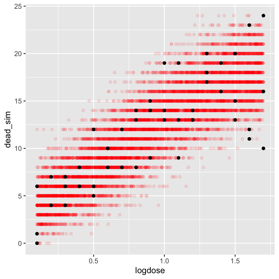

Gaussian error model

We repeat the previous example on the airquality dataset using a log-linear model with a gaussian error term.

airquality <- na.omit(airquality)
glmd <- glm(Ozone ~ Temp, data = airquality, gaussian(link = "log"))

coef(glmd)

## (Intercept)        Temp 
## -1.17546405  0.06124099

b0 <- coef(glmd)[1]
b1 <- coef(glmd)[2]
n <- 10000 # sample size
sigma <- sqrt(summary(glmd)$dispersion)

# create sample of n observations for independent variable X
X <- seq(min(airquality$Temp), max(airquality$Temp), length.out = n) 
Y <- rnorm(n, exp(b0 + b1*X), sd=sigma)

ds.sim <- data.frame(Temp=X, OzoneSim=Y)

ggplot() +
  geom_point(data = ds.sim, aes(x = Temp, y = OzoneSim), alpha = 0.1, col = "red") +
  geom_point(data = airquality, aes(x = Temp, y = Ozone))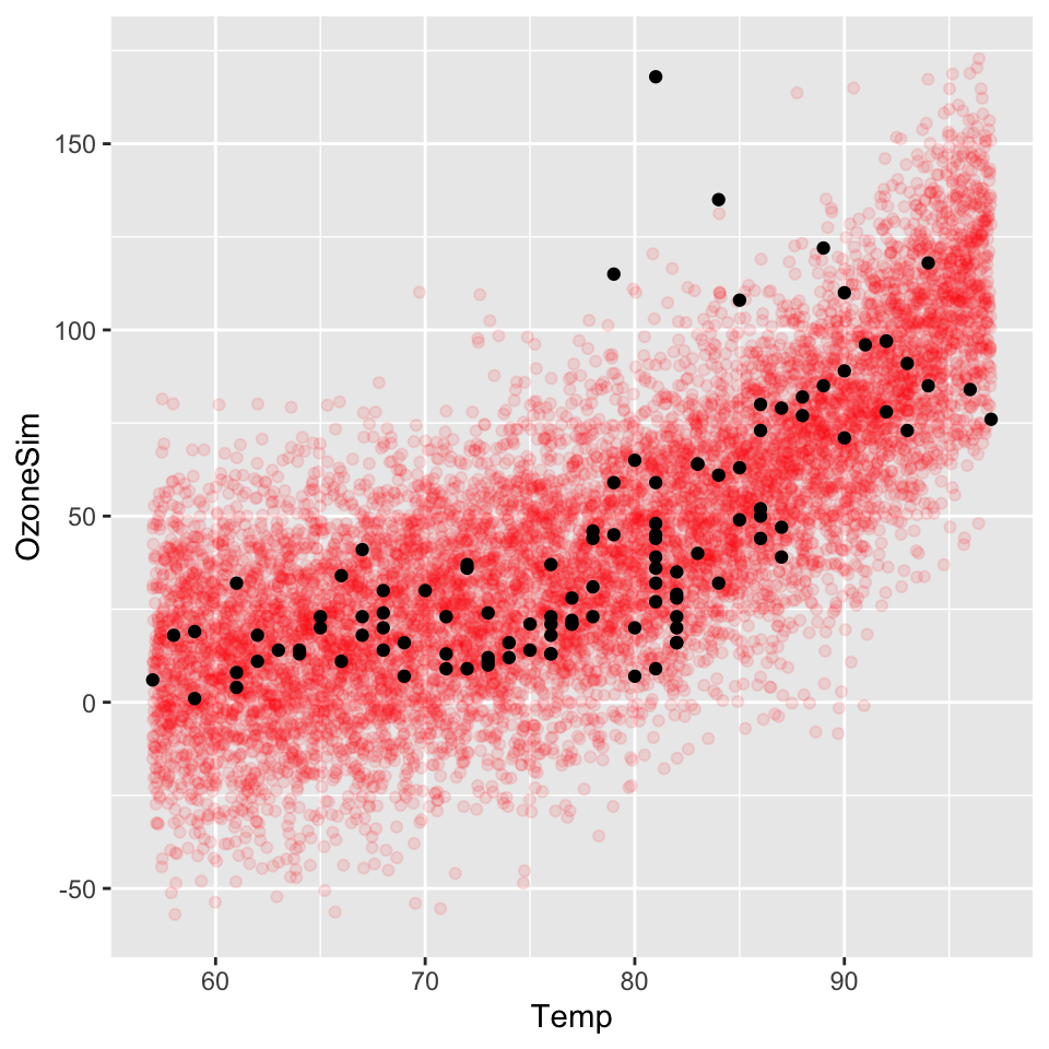

Model checking using DHARmA

There is a package called DHARMa, which implements simulations-based model-checking. The basic steps of the DHARMa workflow are:

Simulate new data from the fitted model
For each observation, calculate the cumulative density function (CDF) of the simulated data
Calculate the residuals as the value of the CDF at the value of the observed data

Assuming the model is correctly specified, all values of the CDF (ranging from 0 to 1) should appear with equal probability. The residuals should thus be uniformely distributed, which we can check by comparing the simulated residuals versus a uniform distribution using QQ-plots.

The package was developed by Florian Hartig, see: https://theoreticalecology.wordpress.com/2016/08/28/dharma-an-r-package-for-residual-diagnostics-of-glmms/

Checking the poisson model fit using DHARMa:

library(DHARMa)

## This is DHARMa 0.4.6. For overview type '?DHARMa'. For recent changes, type news(package = 'DHARMa')

dat <- read.table("Data/bird_counts.txt", sep = ";", header = TRUE)
fit_poisson <- glm(Y ~ relief, data = dat, family = poisson(link = "log"))

sim_poisson <- simulateResiduals(fittedModel = fit_poisson, n = 250)

# Create QQ-plot data
sim_poisson <- data.frame(observed = quantile(sim_poisson$scaledResiduals, p = seq(0, 1, 0.1)),
                          expected = punif(q = seq(0, 1, 0.1),
                                           min(sim_poisson$scaledResiduals),
                                           max(sim_poisson$scaledResiduals)))

ggplot(sim_poisson, aes(x = expected, y = observed)) +
  geom_point() +
  geom_abline(intercept = 0, slope = 1)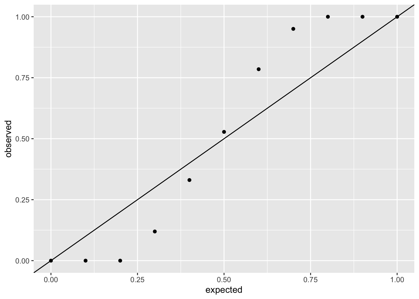

And comparing it to the negative binomial model:

fit_negbin <- glm.nb(Y ~ relief, data = dat, link = "log")

sim_negbin <- simulateResiduals(fittedModel = fit_negbin, n = 250)

# Create QQ-plot data
sim_negbin_resid <- data.frame(observed = quantile(sim_negbin$scaledResiduals, p = seq(0, 1, 0.1)),
                               expected = punif(q = seq(0, 1, 0.1),
                                                min(sim_negbin$scaledResiduals),
                                                max(sim_negbin$scaledResiduals)))

ggplot(sim_negbin_resid, aes(x = expected, y = observed)) +
  geom_point() +
  geom_abline(intercept = 0, slope = 1)

We can also check last week’s logistic regression model:

dat <- read.csv("Data/infestation.csv")
fit_logit <- glm(infested ~ temp_anomaly, data = dat, family = binomial(link = "logit"))

sim_logit <- simulateResiduals(fittedModel = fit_logit, n = 250)

# Create QQ-plot data
sim_logit_resid <- data.frame(observed = quantile(sim_logit$scaledResiduals, p = seq(0, 1, 0.1)),
                              expected = punif(q = seq(0, 1, 0.1),
                                               min(sim_logit$scaledResiduals),
                                               max(sim_logit$scaledResiduals)))

ggplot(sim_logit_resid, aes(x = expected, y = observed)) +
  geom_point() +
  geom_abline(intercept = 0, slope = 1)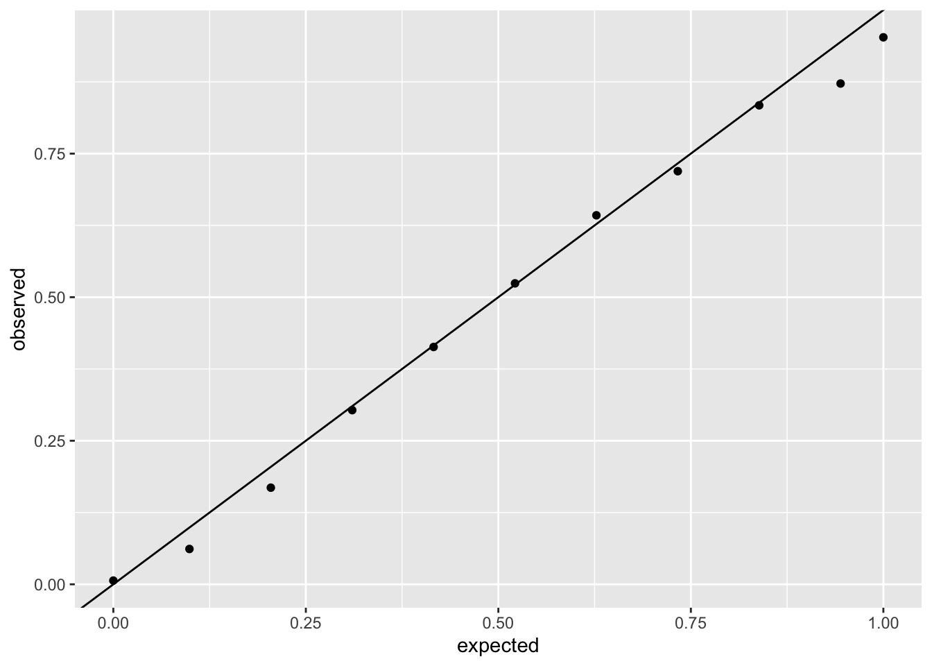

Or the mortality rate model:

dat <- read.table("Data/logistic.txt", sep = "\t", header = TRUE)

fit_logit <- glm(cbind(dead, n - dead) ~ logdose,
                 data = dat, 
                 family = binomial(link = "logit"))

sim_logit <- simulateResiduals(fittedModel = fit_logit, n = 250)

# Create QQ-plot data
sim_logit_resid <- data.frame(observed = quantile(sim_logit$scaledResiduals, p = seq(0, 1, 0.1)),
                              expected = punif(q = seq(0, 1, 0.1),
                                               min(sim_logit$scaledResiduals),
                                               max(sim_logit$scaledResiduals)))

ggplot(sim_logit_resid, aes(x = expected, y = observed)) +
  geom_point() +
  geom_abline(intercept = 0, slope = 1)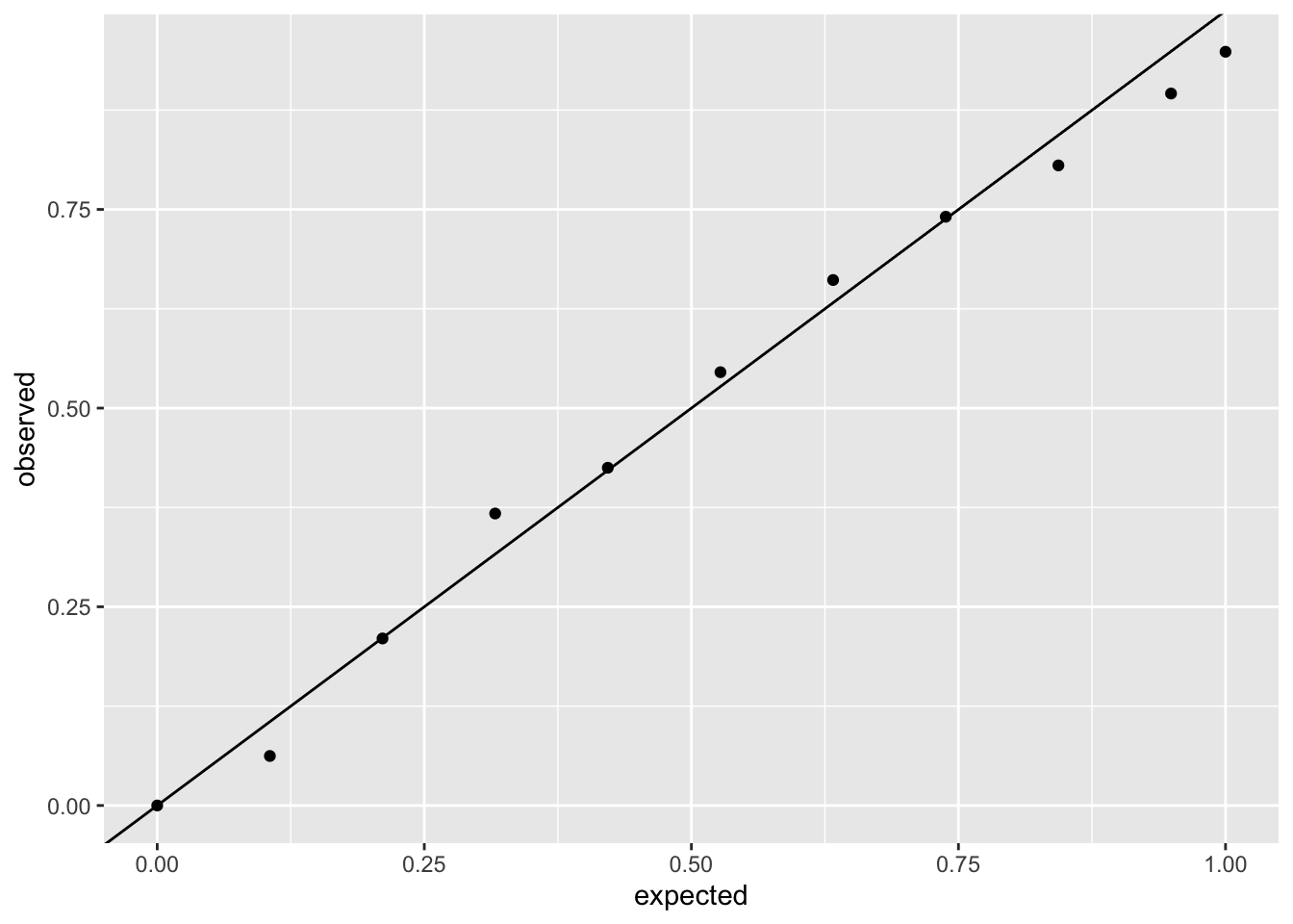

Simulations

Humboldt-Universität zu Berlin | Geography Department

Recap GLMs

Today’s session

Packages

Distributions in R

Probability distribution function

Cummulative distribution function

Inverse cummulative distribution function

Random draws

Simulations

Simulating uncertainty in regression coefficients

Simulating OLS

Confidence and prediction interval

Logistic regression

Poisson regression (Counts)

Tackling overdispersion

Negative binomial GLM

Gaussian error model

Model checking using DHARmA