Continuous predictions
continuous_predictions.RmdExample
Our example uses a simulated test dataset containing an observed
and a predicted
variable. With the aa_predobs function, you can estimate a
suite of error statistics.
pred_errors <- aa_predobs(test$y_obs, test$y_pred, df=T)
pred_errors
#>                       stat
#> bias           0.011944825
#> varratio       0.850698750
#> mse            0.032482187
#> rmse           0.180228152
#> rrmse         35.869406693
#> mlp            0.029772398
#> mla            0.002709789
#> rmlp           0.172546799
#> rmla           0.052055633
#> plp            0.916576155
#> pla            0.083423845
#> sma_intercept  0.086962203
#> sma_slope      0.850698750
#> ols_intercept  0.151910035
#> ols_slope      0.721438134
#> r_squared      0.719194903
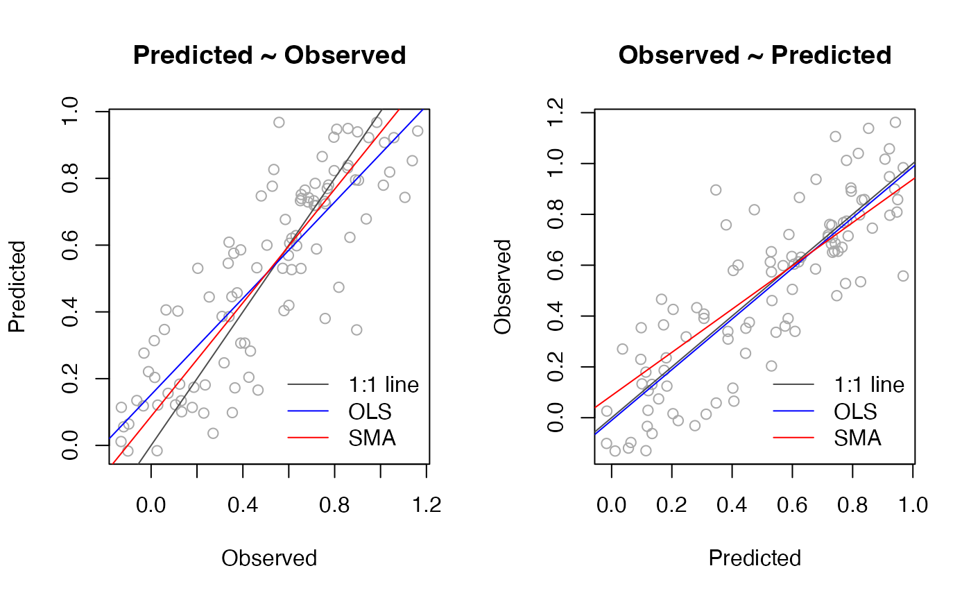
The model had a prediction accuracy of 0.18 (RMSE), which is 35.9% of the mean observation (rRMSE). The bias of 0.01 is negligible. The bias is an estimate of the mean systematic error. However, systematic errors may not be constant across the range of observations. For example, regression models tend to over-predict at low values and under-predict at high values (regression effect). To evaluate potential bias, it makes sense to take a look at the scatterpot. We can also fit a regression line between the predictions and observations, to quantify the bias.
In the literature, you will find three methods for fitting such a regression line to the predictions: 1) ordinary least squares regression (OLS) with the observations on the x-axis and the predictions on the y-axis, 2) OLS with the predictions on the x-axis and the observations on the y-axis, and 3) standardized (=reduced) major axis regression (SMA). OLS fits a line by minimizing the residuals in the y-direction only. In comparison, SMA minimizes the residuals in the x- and y-direction. Consequently, OLS assumes that the x-variable is measured without (or with negligible) error. While this assumption may be reasonable for certain applications, the measurement errors are often not trivial in remote sensing studies. Note, that measurement errors here may include actual instrument errors but also geo-location uncertainties when linking reference data (obtained in the field or high-resolution data) with satellite observations.

Many studies put the observations on the x-axis (Figure, left). Using OLS the estimated slope is 0.721, which suggests a significant overestimation at low values and underestimation at high values. However, method (1) ignores errors in the observations. A number of studies have suggested to reverse the axis (Figure, right). Putting the predictions on the x-axis reduces the regression effect (low and high values tend towards mean). This can be seen in the right figure where the OLS line is close to the 1:1 line. However, method (2) assumes that the predictions are obtained without error, which seems difficult to justify. In comparison, SMA leads to symmetric slope estimates, regardless of the choice of axis. The SMA slope estimate of 0.851 lies between the slopes of the other two methods. Please see Correndo et al. (2021a) for a more detailed description and discussion of the topic.
Error decomposition
Following Correndo et al. (2021a), we partition the prediction error, specifically the MSE, into a systematic and non-systematic component. In our example dataset, the proportion of the random component is PLP=0.92 and the proportion of the systematic component is PLA=0.08.
Equations
| Statistic | Description | Equation |
|---|---|---|
| bias | Bias | |
| Varratio | Variance ratio | |
| MSE | Mean square error (MSE) | |
| RMSE | Root mean square error | |
| rRMSE | Relative RMSE | |
| MLP | Mean Lack of Precision | |
| MLA | Mean Lack of Accuracy | |
| RMLP | Root Mean Lack of Precision | |
| RMLA | Root Mean Lack of Accuracy | |
| PLP | Proportion Lack of Precision | |
| PLA | Proportion Lack of Accuracy | |
| Intercept of standardized major axis regression (SMA) | ||
| Slope of standardized major axis regression (SMA) | ||
| Intercept of ordinary least squares regression (OLS) | ||
| Slope of ordinary least squares regression (OLS) | ||
| Coefficient of determination between predictions and observations |
References
Correndo, A.A., Hefley, T.J., Holzworth, D.P., & Ciampitti, I.A., 2021a. Revisiting linear regression to test agreement in continuous predicted-observed datasets. Agricultural Systems, 192. https://doi.org/10.1016/j.agsy.2021.103194
Correndo, A.A., Hefley, T., Holzworth, D., Ciampitti, I.A., 2021b. R-Code Tutorial: Revisiting linear regression to test agreement in continuous predicted-observed datasets. Harvard Dataverse V3. https://doi.org/10.7910/DVN/EJS4M0.
Kuhn, M., & Johnson, K., 2013. Applied predictive modeling. New York: Springer. https://link.springer.com/book/10.1007/978-1-4614-6849-3
Pauwels, V.R.N., Guyot, A., & Walker, J.P., 2019. Evaluating model results in scatter plots: A critique. Ecological Modelling, 411. https://users.monash.edu.au/~jpwalker/papers/em19.pdf
Piñeiro, G., Perelman, S., Guerschman, J.P., & Paruelo, J.M., 2008. How to evaluate models: Observed vs. predicted or predicted vs. observed? Ecological Modelling, 216, 316-322. https://doi.org/10.1016/j.ecolmodel.2008.05.006