Getting started
getting-started.RmdInstall package
# install devtools packages
if (!require(devtools)) install.packages("devtools")

# load devtools package
library(devtools)

# install mapac package from gitlab
install_git("https://scm.cms.hu-berlin.de/pflugmad/mapac.git", quiet=F, force=T)

# Additional packages
install.packages(c("ggplot2", "tidyr", "gt"))
Load package and example
library(mapac)
library(gt)

# load example data from Stehman (2014)

exdata <- aa_examples("stehman2014")
exdata
#> $reference
#>  [1] "A" "A" "A" "A" "A" "C" "B" "A" "B" "C" "A" "B" "B" "B" "B" "B" "A" "A" "B"
#> [20] "B" "C" "C" "C" "C" "C" "D" "D" "B" "B" "A" "D" "D" "D" "D" "D" "D" "D" "C"
#> [39] "C" "B"
#>
#> $map
#>  [1] "A" "A" "A" "A" "A" "A" "A" "B" "B" "B" "A" "B" "B" "B" "B" "B" "B" "B" "B"
#> [20] "B" "B" "B" "C" "C" "C" "C" "C" "C" "B" "B" "D" "D" "D" "D" "D" "D" "D" "D"
#> [39] "D" "D"
#>
#> $stratum
#>  [1] "1" "1" "1" "1" "1" "1" "1" "1" "1" "1" "2" "2" "2" "2" "2" "2" "2" "2" "2"
#> [20] "2" "3" "3" "3" "3" "3" "3" "3" "3" "3" "3" "4" "4" "4" "4" "4" "4" "4" "4"
#> [39] "4" "4"
#>
#> $h
#> [1] "1" "2" "3" "4"
#>
#> $N_h
#> [1] 40000 30000 20000 10000
#>
#> $citation
#> [1] "Stehman, S. V., 2014. Estimating area and map accuracy for stratified random sampling when the strata are different from the map classes. Int. J. Remote Sens. 35, 4923-4939."
In the example from Stehman (2014), the sampling strata are different from the map strata. To illustrate the point, we extract the stratum labels, the map labels, and the reference labels into three vectors below. The stratum, map, and reference labels can be of type numeric, character, or factor. However, reference and map labels should be of the same type. Use factors if you want to control the class order of the resulting confusion matrices and graphs.
strata <- exdata[["stratum"]]
ref <- exdata[["reference"]]
map <- exdata[["map"]]
To estimate map accuracy and area we can use the
aa_stratified() function. The function takes the three
vectors above and information on the stratum sizes N_h,
e.g. in the form of number of pixels, area, or area proportion. In our
example, there are 4 strata where h = {"1", "2", "3", "4"}.
Thus, h is a vector of the stratum labels that correspond
to the stratum sizes N_h and the stratum samples
strata.
result <-  aa_stratified(strata, ref, map,
                         h=exdata[["h"]],
                         N_h=exdata[["N_h"]])
The result is a list with the following content:
$cm: the adjusted confusion matrix in counts
$cmp: the adjusted confusion matrix in area proportion (sums to 1).
$stats: User’s (ua) and Producer’s (pa) accuracy and the corresponding standard errors (se) for each class.
$accuracy: Overall accuracy and its standard error
$area: estimated area proportion and standard errors for each class
result
#> $cm
#>     A    B   C   D
#> A 9.2  1.6 1.6 0.0
#> B 4.8 10.8 3.2 0.0
#> C 0.0  0.8 2.4 1.6
#> D 0.0  0.4 0.8 2.8
#>
#> $cmp
#>      A    B    C    D
#> A 0.23 0.04 0.04 0.00
#> B 0.12 0.27 0.08 0.00
#> C 0.00 0.02 0.06 0.04
#> D 0.00 0.01 0.02 0.07
#>
#> $stats
#>   class        ua     ua_se        pa     pa_se        f1      f1_se
#> 1     A 0.7419355 0.1645627 0.6571429 0.1477318 0.6969697 0.11034620
#> 2     B 0.5744681 0.1248023 0.7941176 0.1165671 0.6666667 0.09354009
#> 3     C 0.5000000 0.2151657 0.3000000 0.1504438 0.3750000 0.13219833
#> 4     D 0.7000000 0.1527525 0.6363636 0.1623242 0.6666667 0.11284328
#>
#> $accuracy
#> [1] 0.63000000 0.08465617
#>
#> $fpc
#> [1] 1 1 1 1
#>
#> $area
#>   class proportion proportion_se
#> 1     A       0.35    0.08225975
#> 2     B       0.34    0.07586538
#> 3     C       0.20    0.06429101
#> 4     D       0.11    0.03073181
Export results
You can easily export the results as tables in text files.
write.csv(result$cmp, "my_confusion_matrix.csv")Visualize confusion matrices
There are a few functions to facilitate visualization and reporting.
For example, with aa_confusion_matrix_gtable() you can
create confusion matrices with conditional formats. You can save the
table in HTML format via the out_file argument.
cm <- aa_confusion_matrix_gtable(result)
cm| Map class |
Reference class (area %)
|
Σ
|
Accuracy
|
||||||
|---|---|---|---|---|---|---|---|---|---|
| A | B | C | D | Map | Ref. | Producer's | User's | F-score | |
| A | 23.00 | 4.00 | 4.00 | 0.00 | 31.00 | 35.00 | 65.71 ± 14.77 | 74.19 ± 16.46 | 69.70 ± 11.03 |
| B | 12.00 | 27.00 | 8.00 | 0.00 | 47.00 | 34.00 | 79.41 ± 11.66 | 57.45 ± 12.48 | 66.67 ± 9.35 |
| C | 0.00 | 2.00 | 6.00 | 4.00 | 12.00 | 20.00 | 30.00 ± 15.04 | 50.00 ± 21.52 | 37.50 ± 13.22 |
| D | 0.00 | 1.00 | 2.00 | 7.00 | 10.00 | 11.00 | 63.64 ± 16.23 | 70.00 ± 15.28 | 66.67 ± 11.28 |
Overall accuracy = 63 ± 8.47 |
|||||||||
cm <- aa_confusion_matrix_gtable(result, type="proportion",
                                 title="Confusion matrix (area proportion)")
cm| Confusion matrix (area proportion) | |||||||||
| Map class |
Reference class (area proportion)
|
Σ
|
Accuracy
|
||||||
|---|---|---|---|---|---|---|---|---|---|
| A | B | C | D | Map | Ref. | Producer's | User's | F-score | |
| A | 0.23 | 0.04 | 0.04 | 0.00 | 0.31 | 0.35 | 65.71 ± 14.77 | 74.19 ± 16.46 | 69.70 ± 11.03 |
| B | 0.12 | 0.27 | 0.08 | 0.00 | 0.47 | 0.34 | 79.41 ± 11.66 | 57.45 ± 12.48 | 66.67 ± 9.35 |
| C | 0.00 | 0.02 | 0.06 | 0.04 | 0.12 | 0.20 | 30.00 ± 15.04 | 50.00 ± 21.52 | 37.50 ± 13.22 |
| D | 0.00 | 0.01 | 0.02 | 0.07 | 0.10 | 0.11 | 63.64 ± 16.23 | 70.00 ± 15.28 | 66.67 ± 11.28 |
Overall accuracy = 63 ± 8.47 |
|||||||||
If you have long class names, it may be useful to use numbers in the column header.
cm <- aa_confusion_matrix_gtable(result, colNumbering = T, zero.rm=T)
cm| Map class |
Reference class (area %)
|
Σ
|
Accuracy
|
||||||
|---|---|---|---|---|---|---|---|---|---|
| 1 | 2 | 3 | 4 | Map | Ref. | Producer's | User's | F-score | |
| A | 1 | 23.00 | 4.00 | 4.00 | 0.00 | 31.00 | 35.00 | 65.71 ± 14.77 | 74.19 ± 16.46 | 69.70 ± 11.03 |
| B | 2 | 12.00 | 27.00 | 8.00 | 0.00 | 47.00 | 34.00 | 79.41 ± 11.66 | 57.45 ± 12.48 | 66.67 ± 9.35 |
| C | 3 | 0.00 | 2.00 | 6.00 | 4.00 | 12.00 | 20.00 | 30.00 ± 15.04 | 50.00 ± 21.52 | 37.50 ± 13.22 |
| D | 4 | 0.00 | 1.00 | 2.00 | 7.00 | 10.00 | 11.00 | 63.64 ± 16.23 | 70.00 ± 15.28 | 66.67 ± 11.28 |
Overall accuracy = 63 ± 8.47 |
|||||||||
Alternatively, you can provide a different set of class names.
cm <- aa_confusion_matrix_gtable(result, colNumbering = T,
                                 classLabels=c("u", "v", "x", "y"))
cm| Map class |
Reference class (area %)
|
Σ
|
Accuracy
|
||||||
|---|---|---|---|---|---|---|---|---|---|
| 1 | 2 | 3 | 4 | Map | Ref. | Producer's | User's | F-score | |
| u | 1 | 23.00 | 4.00 | 4.00 | 0.00 | 31.00 | 35.00 | 65.71 ± 14.77 | 74.19 ± 16.46 | 69.70 ± 11.03 |
| v | 2 | 12.00 | 27.00 | 8.00 | 0.00 | 47.00 | 34.00 | 79.41 ± 11.66 | 57.45 ± 12.48 | 66.67 ± 9.35 |
| x | 3 | 0.00 | 2.00 | 6.00 | 4.00 | 12.00 | 20.00 | 30.00 ± 15.04 | 50.00 ± 21.52 | 37.50 ± 13.22 |
| y | 4 | 0.00 | 1.00 | 2.00 | 7.00 | 10.00 | 11.00 | 63.64 ± 16.23 | 70.00 ± 15.28 | 66.67 ± 11.28 |
Overall accuracy = 63 ± 8.47 |
|||||||||
Visualize class accuracies
aa_class_accuracy_plot(result)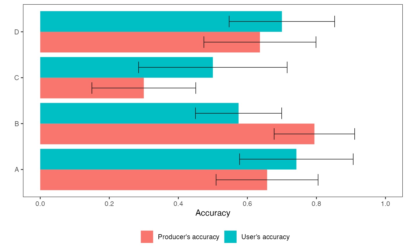
You can save the ggplot as follows:
ggsave('class_accuracy_.png', p, width=9, height=6, units="cm", dpi=300, scale=2)