Lab 01: Mono Lake
Submit the lab before May 9th 2024, 20:00
Introduction
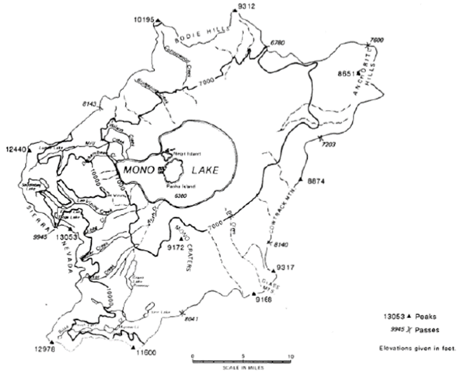
This assignment represents the first case study in which we will use Vensim as a tool to create a first process-model using the tools and techniques learned last week. This week, we want you to build a hydrological model of the Mono Lake drainage basin (Figure 1). The Mono Lake drainage basin is located 190 miles east of San Francisco. It is surrounded by the Sierra Nevada mountains, Bodie Hills, Mono Craters, Anchorite Hills, and Cowtrack Mountain. The climate is of high-altitude Mediterranean type with great seasonal and annual precipitation variability. Within the basin, all surface water (as well as groundwater) is derived from precipitation over the basin itself (collected by small streams), and predominantly from precipitation over the Sierra Mountains, both draining into the Mono basin and towards Mono Lake; it is a hydro-geographically closed region. The Mono Lake dominates the center of the basin and is a terminal lake. However, runoff generated in the Sierra Mountains is used to meet freshwater demands in the greater Los Angeles area. That is why in most years a substantial share, and possibly almost the entire flow from the Sierra Nevada is diverted towards Los Angeles. Also have a look at https://www.monolake.org/
Exercise I: Implementation of the Mono Lake system model in Vensim
In Figure 2 you find a stock-and-flow diagram of the Mono Lake hydrological model. In this first task, we ask you to implement this model in Vensim using the knowledge you gained in last week’s exercise. For the implementation, remember that the symbology in Vensim is slightly different from the one used below. Specifically, in the below example circles  represent auxiliary variables which in Vensim are incorporated using the button
  . The
. The  symbol below are flows, built in Vensim as
  . Stocks and links below have the same notation in Vensim
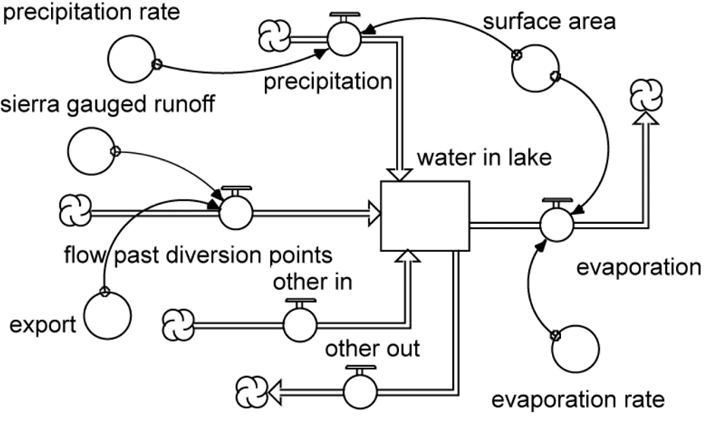
After you implement the model in Vensim, you need to parameterize all stocks and flows. Do this using the parameters provided in Table 1, i.e., by filling the initial values and equations if needed. The units in Vensim (i.e., in the variable information that appears once you click on an object with the equation tool  ) are only for visual purposes and will only appear on graphs – this means, that before running any simulation you will need to check whether the units between stocks and flows are provided at the same scale. If they do differ in scale (e.g., hectare vs. acre) you will need to convert the units manually. In our example here, no conversion is necessary. Yet, the units provided there will give you an idea on how to set some of the equations.
| Parameter | Value | Unit of measurement |
|---|---|---|
| Surface Area | 39 | KA (1000 acres) |
| Reservoir volume | 2,228 | KAF (1000 acre-foot) |
| Gauged runoff from the Sierra Mountain range | 150 | \(KAF *yr^-1\) |
| Other inflows | 47.6 | \(KAF *yr^-1\) |
| Diversion of water (export) towards the Los Angeles agglomeration | 100 | \(KAF *yr^-1\) |
| Other outflows (accumulated total) | 33.6 | \(KAF *yr^-1\) |
| Precipitation rate | 0.67 | \(ft *yr^-1\) |
| Evaporation rate | 3.75 | \(ft *yr^-1\) |
Once you set up your model and provided all parameters, we want to you to run a simulation from 1990 to 2030 in time intervals of 1 year (Δt = 1). Go to the Model –> Settings and check whether Euler is selected as integration technique. In the same menu, under “Time Bounds” the box Save results every TIME STEP should be ticked (this is a technical detail concerning how the model file is stored – for the moment, we will neglect this detail). After the simulation, carefully examine the output and answer the questions below in moodle.
Exercise II: Implementing relationships between variables inside the model
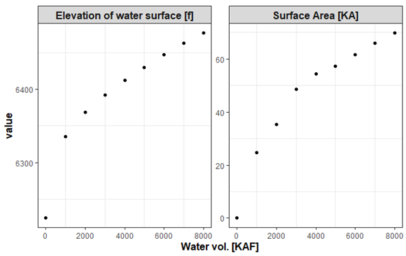
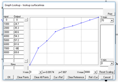
The first version of the model has clearly some issues, and in this exercise we will modify the model in the way by implementing a response of the surface area (i.e., changes therein) to changes in the stock water volumes. In Vensim, one can do that through the integration of so-called look-up tables into the model. In a look-up table one can establish relationships between two (or more) variables, e.g., between water volume and surface. You can find the required input for such a look-up table in Table 2 and the corresponding visualization in Figure 3.
| Water volume in reservoir [KAF] | Surface area [KA] | Elevation of water surface [ft a.s.l.] |
|---|---|---|
| 0 | 0 | 6224 |
| 1000 | 24.7 | 6335 |
| 2000 | 35.3 | 6369 |
| 3000 | 48.6 | 6392 |
| 4000 | 54.3 | 6412 |
| 5000 | 57.2 | 6430 |
| 6000 | 61.6 | 6447 |
| 7000 | 66.0 | 6463 |
| 8000 | 69.8 | 6477 |
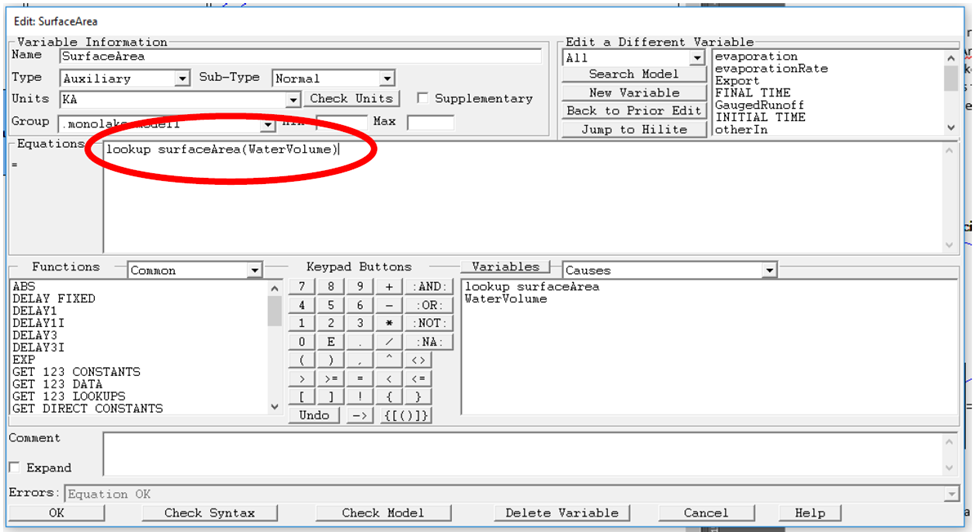
To implement such a lookup table in Vensim you will need to add a variable to the model that will be used as a lookup (here called: lookup_surfaceArea). Open the equations dialog for this variable (using the ) button) and change the type of the variable to LookUp (Figure 4).
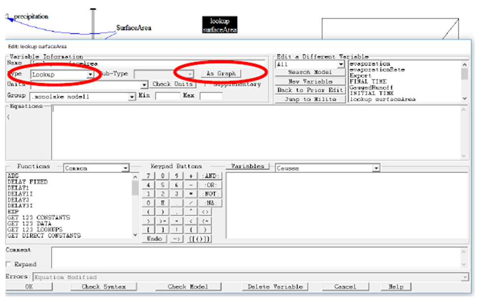
Now you need to establish the relationship between the variable surface area and water volume for this lookup. You do this, by navigating to the As Graph menu and by entering the values into the table that is shown. Make sure you assign the variable water volume as x (i.e., Input) and surface area as y (i.e., Output). Vensim will directly translate these values into the corresponding visualization using linear interpolation between the values (Figure 5). Click okay and you’ll see that the information that you just entered is encoded in the Equations text box. After that, close the ) dialog.
Now we need to make changes to the model structure in order to make use of the look-up that we just created. The variable SurfaceArea now contains values that correspond to the actual surface area of the lake depending on the actual water volume – all provided through the lookup-function that we built. Now, all is left is to add a link between the variable WaterVolume`` and the variableSurfaceArea``:
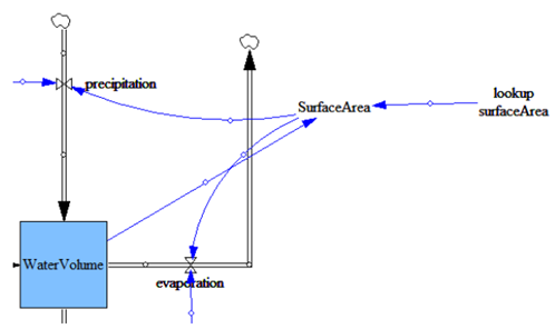
WaterVolume`` toSurfaceArea.``.
Next, change the equation of the variable `SurfaceArea`` as indicated below. This function will pass the current water volume to the look-up variable which will return the corresponding surface area which then is used to determine evaporation and precipitation. Use a table or a graph module to visualize the changes in the surface area.
Now, that we are all set. Run the model for the period 1990-2090 using a time interval of 1 year applying Euler’s integration (like in exercise I). Based on your outcomes, answer the questions below.
Before we proceed to exercise 3, I want you to make one more modification to the model. Specifically, please implement now the water surface elevation (in ft. a.s.l.) into the model using a look-up table as before. This variable, which represents the elevation of the water surface is also function of the lake’s water level. Re-run the experiment and answer the question below. After that, continue to exercise 3.
Exercise III: Salinity and its impact on evaporation
Evaporation is not only dependent on the surface area of Mono Lake, but it additionally depends on the salinity and the density of the lake’s water. For example, highly saline water tends to evaporate more slowly – which means that the higher the salinity of the water is, the lower is the effective evaporation. The density of water, on the other hand, depends on the number of solids that are dissolved in water. The effect of increasing density can be expressed by applying the formula of specific gravity \(SG\):
\[ SG = \frac{V_{reservoir} * \rho_{freshwater} + m_{dissolved}}{V_{reservoir} * \rho_{freshwater}} \] where \(V_{reservoir}\) is the water volume (KAF), \(\rho_{freshwater}\) corresponds to the freshwater reference (density) fixed at 1.359 Mio. t per KAF, and where \(m_{dissolved}\) is the total amount of solids dissolved in the lake, which equals here to 230 Mio t. The relationship between specific gravity (without unit) and evaporation, expressed through the effective evaporation rate, is shown in Table 3.
| Specific gravity | Effective evaporation rate coefficient |
|---|---|
| 1.00 | 1.00 |
| 1.05 | 0.963 |
| 1.10 | 0.962 |
| 1.15 | 0.880 |
| 1.20 | 0.833 |
| 1.25 | 0.785 |
| 1.30 | 0.737 |
| 1.35 | 0.688 |
| 1.40 | 0.640 |
Your task now is to implement this additional detail to your model using the techniques you learned in the previous exercises. After that, re-run the simulation for the period 1990-2090. Once you have done this, please answer the questions below.
Exercise IV: Mono Lake policy questions
After implementing the changes related to evaporation, the model can now be used to assess the impact of various policies, such as for managing water as a resource. Likewise, the model could also be used to explore impacts of global megatrends. Consider a sea-level elevation of 6340 ft asl. to be set as a policy threshold level, below which no further water from the lake is allowed to be drained. Implement this threshold as an auxiliary variable and include it into the graph that shows the elevation.
Simulate a system, in which export of water is allowed if the above-mentioned threshold level is exceeded and disallowed otherwise. To do that, you’ll have to extend your model for this by incorporating the threshold level in a meaningful way.