Table manipulation

Table manipulation#

Pandas, short for Python Data Analysis Library, is a modern, powerful and feature rich library that is designed for doing data analysis in Python. Here, we will cover some basic Pandas that will allow you to store results in table format, do some basic table operations, visualization, and to read and write tables to files. You will find more information online in the Pandas Tutorials and in chapter 3 of the Python Data Science Handbook [VanderPlas, 2016].

import pandas as pd
pd.__version__

'2.1.1'

DataFrame#

The main pandas data structure is a table format called DataFrame. A DataFrame contains an Index and it contains columns. Columns are one-dimensional arrays of a single type called Series. A DataFrame can be created from a:

single Series object
list of dicts
dictionary of Series objects
two-dimensional NumPy array
NumPy structured array

mySeries = pd.Series(['London', 'Paris', 'Berlin'], name='City', dtype='string')
cities = pd.DataFrame({"City": mySeries, "Population": [8.8, 2.2, 3.6]})
cities

	City	Population
0	London	8.8
1	Paris	2.2
2	Berlin	3.6

DataFrames have the following attributes: dtypes, shape, index, columns, values, empty.

cities.columns

Index(['City', 'Population'], dtype='object')

cities.dtypes

City          string[python]
Population           float64
dtype: object

cities.shape

(3, 2)

cities.values

array([['London', 8.8],
       ['Paris', 2.2],
       ['Berlin', 3.6]], dtype=object)

Reading and writing#

The pandas library can read a variety of data formats using pandas.read_*(), including CSV, JSON, HTML, HDF5, Excel, SQL, SPSS, SAS, etc.:

fname = '../data/pandas/airquality.csv'
airq = pd.read_csv(fname, index_col=0)
airq.head()

	Ozone	Solar	Wind	Temp	Month	Day
ID
101	41.0	190.0	7.4	67	5	1
102	36.0	118.0	8.0	72	5	2
103	12.0	149.0	12.6	74	5	3
104	18.0	313.0	11.5	62	5	4
105	NaN	NaN	14.3	56	5	5

The DataFrame object contains to_*() methods to write it to a file or database, e.g. airq.to_csv(out_filename).

Inspect DataFrame#

DataFrames have several methods that are useful for inspection: head(), tail(), and describe()

airq.describe()

	Ozone	Solar	Wind	Temp	Month	Day
count	116.000000	146.000000	153.000000	153.000000	153.000000	153.000000
mean	42.129310	185.931507	9.957516	77.882353	6.993464	15.803922
std	32.987885	90.058422	3.523001	9.465270	1.416522	8.864520
min	1.000000	7.000000	1.700000	56.000000	5.000000	1.000000
25%	18.000000	115.750000	7.400000	72.000000	6.000000	8.000000
50%	31.500000	205.000000	9.700000	79.000000	7.000000	16.000000
75%	63.250000	258.750000	11.500000	85.000000	8.000000	23.000000
max	168.000000	334.000000	20.700000	97.000000	9.000000	31.000000

Access values#

Select columns#

airq.Ozone

ID
  41.0
  36.0
  12.0
  18.0
   NaN
       ... 
  30.0
   NaN
  14.0
  18.0
  20.0
Name: Ozone, Length: 153, dtype: float64

…or using a name or a list of names.

airq["Ozone"].head()

ID
  41.0
  36.0
  12.0
  18.0
   NaN
Name: Ozone, dtype: float64

airq[["Ozone", "Solar"]].head()

	Ozone	Solar
ID
101	41.0	190.0
102	36.0	118.0
103	12.0	149.0
104	18.0	313.0
105	NaN	NaN

Select rows#

We can extract rows (called slicing) from a date frame using indexing similar to indexing lists and tuples, where the first index is being inclusive and the last exclusive.

airq[2:4]

	Ozone	Solar	Wind	Temp	Month	Day
ID
103	12.0	149.0	12.6	74	5	3
104	18.0	313.0	11.5	62	5	4

Rows and columns#

To extract rows and columns, we need to chain the commands pulling the columns and then the rows or vice versa (order does not matter).

airq[["Ozone", "Solar"]][2:4]

	Ozone	Solar
ID
103	12.0	149.0
104	18.0	313.0

Indexing#

The loc attribute allows indexing and slicing that always references the explicit index
The iloc attribute allows indexing and slicing that always references the implicit Python-style index
The ix attribute was a hybrid of the two. It is now depreciated.

Using the iloc indexer, we can index the underlying array as if it is a simple NumPy array (using the implicit Python-style index), but the DataFrame index and column labels are maintained in the result:

airq.iloc[1:3, 2:4]

	Wind	Temp
ID
102	8.0	72
103	12.6	74

Similarly, using the loc indexer we can index the underlying data in an array-like style but using the explicit row index and column indices:

airq.loc[100:102, ["Wind", "Temp"]]

	Wind	Temp
ID
101	7.4	67
102	8.0	72

Masking#

There are a couple extra indexing conventions that might seem at odds with the preceding discussion, but nevertheless can be very useful in practice. First, while indexing refers to columns, slicing refers to rows. We’ve already used numerical ranges for slices. Also, boolean masking operations work for selecting rows.

airq[(airq.Ozone > 15) & (airq.Ozone < 18)]

	Ozone	Solar	Wind	Temp	Month	Day
ID
112	16.0	256.0	9.7	69	5	12
182	16.0	7.0	6.9	74	7	21
195	16.0	77.0	7.4	82	8	3
243	16.0	201.0	8.0	82	9	20

Asign new column#

import numpy as np
airq["logOzone"]  = np.log(airq.Ozone)
airq.head()

	Ozone	Solar	Wind	Temp	Month	Day	logOzone
ID
101	41.0	190.0	7.4	67	5	1	3.713572
102	36.0	118.0	8.0	72	5	2	3.583519
103	12.0	149.0	12.6	74	5	3	2.484907
104	18.0	313.0	11.5	62	5	4	2.890372
105	NaN	NaN	14.3	56	5	5	NaN

Methods#

You can do masking and other useful things directly via methods of Series and DataFrames., e.g.

airq.Ozone.between(15, 18)
airq.Month.isin([5, 8])
airq.Month.astype(“string”)

airq.isna().sum()

Ozone       37
Solar        7
Wind         0
Temp         0
Month        0
Day          0
logOzone    37
dtype: int64

Simple aggregation functions include mean(), median(), min(), max(), and std().

airq['Ozone'].mean()

42.12931034482759

Grouping#

Sometimes we want to apply aggregation functions for individual factors separately.

airq.groupby('Month')

<pandas.core.groupby.generic.DataFrameGroupBy object at 0x11645e300>

Sometimes we want to apply aggregation functions for individual factors separately.

airq.groupby('Month').mean()

	Ozone	Solar	Wind	Temp	Day	logOzone
Month
5	23.615385	181.296296	11.622581	65.548387	16.0	2.812076
6	29.444444	190.166667	10.266667	79.100000	15.5	3.236673
7	59.115385	216.483871	8.941935	83.903226	16.0	3.883834
8	59.961538	171.857143	8.793548	83.967742	16.0	3.845345
9	31.448276	167.433333	10.180000	76.900000	15.5	3.218795

Groupby comes with additional aggregation methods that provide more flexibility: aggregate(), filter(), transform(), and apply().

airq.groupby('Month').aggregate(["min", "max", "mean"])

	Ozone			Solar			Wind			Temp			Day			logOzone
	min	max	mean	min	max	mean	min	max	mean	min	max	mean	min	max	mean	min	max	mean
Month
5	1.0	115.0	23.615385	8.0	334.0	181.296296	5.7	20.1	11.622581	56	81	65.548387	1	31	16.0	0.000000	4.744932	2.812076
6	12.0	71.0	29.444444	31.0	332.0	190.166667	1.7	20.7	10.266667	65	93	79.100000	1	30	15.5	2.484907	4.262680	3.236673
7	7.0	135.0	59.115385	7.0	314.0	216.483871	4.1	14.9	8.941935	73	92	83.903226	1	31	16.0	1.945910	4.905275	3.883834
8	9.0	168.0	59.961538	24.0	273.0	171.857143	2.3	15.5	8.793548	72	97	83.967742	1	31	16.0	2.197225	5.123964	3.845345
9	7.0	96.0	31.448276	14.0	259.0	167.433333	2.8	16.6	10.180000	63	93	76.900000	1	30	15.5	1.945910	4.564348	3.218795

Append#

Append rows#

The stack two data.frames together by row, use the concat() function. Note append() will be depreciated in future versions of pandas.

pd.concat([airq.head(2), airq.tail(2)])

	Ozone	Solar	Wind	Temp	Month	Day	logOzone
ID
101	41.0	190.0	7.4	67	5	1	3.713572
102	36.0	118.0	8.0	72	5	2	3.583519
252	18.0	131.0	8.0	76	9	29	2.890372
253	20.0	223.0	11.5	68	9	30	2.995732

Append columns#

The concat() function can also be used to stack columns of DataFrames together. The row index is preserved with an outer join by default.

pd.concat([airq.head(2), airq.tail(2)], axis=1)

	Ozone	Solar	Wind	Temp	Month	Day	logOzone	Ozone	Solar	Wind	Temp	Month	Day	logOzone
ID
101	41.0	190.0	7.4	67.0	5.0	1.0	3.713572	NaN	NaN	NaN	NaN	NaN	NaN	NaN
102	36.0	118.0	8.0	72.0	5.0	2.0	3.583519	NaN	NaN	NaN	NaN	NaN	NaN	NaN
252	NaN	NaN	NaN	NaN	NaN	NaN	NaN	18.0	131.0	8.0	76.0	9.0	29.0	2.890372
253	NaN	NaN	NaN	NaN	NaN	NaN	NaN	20.0	223.0	11.5	68.0	9.0	30.0	2.995732

To ignore row indices when stacking columns, you need to clear them prior to calling pd.concat().

df1 = airq.head(2).copy().reset_index(drop=True)
df2 = airq.tail(2).copy().reset_index(drop=True)
pd.concat([df1, df2], axis=1)

	Ozone	Solar	Wind	Temp	Month	Day	logOzone	Ozone	Solar	Wind	Temp	Month	Day	logOzone
0	41.0	190.0	7.4	67	5	1	3.713572	18.0	131.0	8.0	76	9	29	2.890372
1	36.0	118.0	8.0	72	5	2	3.583519	20.0	223.0	11.5	68	9	30	2.995732

Merge#

Pandas implements several ways of combining datasets via the pd.merge() function and the join()methods of Series and DataFrames.

The pd.merge() function implements one-to-one, many-to-one, and many-to-many joins.

The pd.merge() function joins based on column names and not the Index. The column names can be explicitly defined via the keywords on, left_on, and right_on.

Copy#

# Shallow copy
shallow_copy = airq

# Deep copy
deep_copy = airq.copy()

Visualization#

matplotlib#

%matplotlib inline
import matplotlib.pyplot as plt
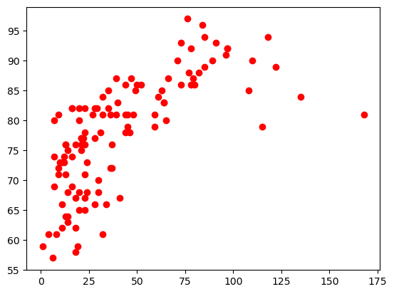
plt.plot(airq.Ozone, airq.Temp, 'or')
plt.show()

../_images/5a15bfac30789211b0dffdc3180878a5ffe659c71e524e1d19716d252c296131.png

Pandas#

Pandas provides visualization tools built on top of matplotlib. Hence, you still need to import matplotlib’s pyplot. You can read more in the pandas reference guide here. There are two ways to use pandas for plotting:

via plot() methods for Series and DataFrames.
via the plotting module pandas.plotting.

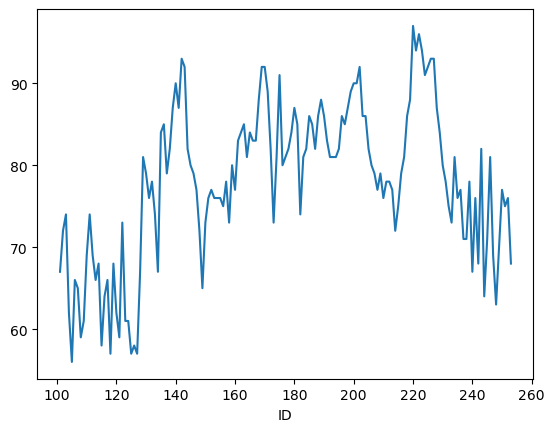
By default plot() shows a line graph using the row indices a x-axis and the columns as data lines:

airq.Temp.plot()
plt.show()

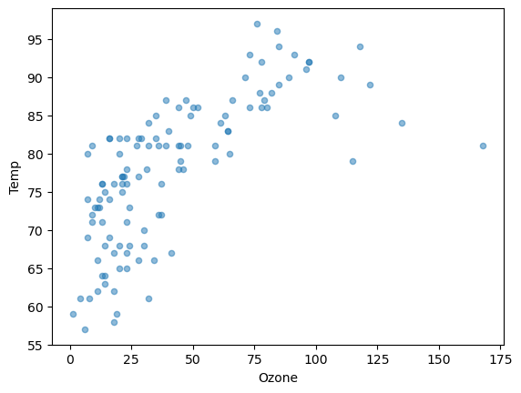
../_images/cb94c3d23478c21b3c3981a3672e1b08318a2111ee0308165fef2ca0c8ced971.png

You can create other plots using the methods DataFrame.plot.kind or provide the kind keyword argument to the plot() method:

airq.plot.scatter(x="Ozone", y="Temp", alpha=0.5)
plt.show()

../_images/b11d5703ef6b3757bd9f72e06812b9e440cce323a9367dab8eefcebd7a8ea9d5.png