Array manipulation#
Arrays are the underlying data structure of raster data. Therefore, understanding how to manipulate arrays is important if you want work with raster data. There are a number of Python packages that provide you with functions that do very specific, pre-determined things with raster data. We will use some of them later in the course. Here, you learn how to work with arrays directly and possibly create your own raster manipulation functions.
The Python package that provides arrays and functions to manipulate arrays is called NumPy. NumPy itself is written in C and therefore fast compared to pure Python code. For a much better description of NumPy, please carefully read Chapter 2 of the Python Data Science Handbook [VanderPlas, 2016].
It is customary to import numpy with the alias np:
import numpy as np
np.__version__
'1.26.0'
Array creation#
You can create an array from a Python list object.
a = np.array([1, 4, 2, 5, 3])
a
array([1, 4, 2, 5, 3])
Because the list contained only integer values, array a is of type integer (64 bits). You can see the data type, by printing the dtype property of the array object. Change the content of the array below and see how the data type changes. For example, change the last element from 3 to 3.0.
a2 = np.array([1, 4, 2, 5, 3])
a2.dtype
dtype('int64')
Usually, it is best to define the data type explicitly upon creation. The code below creates an array of floating point numbers. See the numpy documentation for a list of numpy data types.
a3 = np.array([1, 4, 2, 5, 3], dtype=np.float64)
a3.dtype
dtype('float64')
Numpy provides a number of functions for creating arrays by only defining the dimensions and the fill value.
np.zeros(10, dtype=np.int16)
array([0, 0, 0, 0, 0, 0, 0, 0, 0, 0], dtype=int16)
np.ones(10, dtype=np.int16)
array([1, 1, 1, 1, 1, 1, 1, 1, 1, 1], dtype=int16)
np.arange(start=0, stop=20, step=2)
array([ 0, 2, 4, 6, 8, 10, 12, 14, 16, 18])
The function numpy.full() requires two arguments. The first argument specifies the dimensions (as an integer, list or tuple). The second argument specifies the fill value. The order of the dimensions (shape) for a two-dimensional array are [rows, columns], and with a three dimensional array [bands, rows, columns]. Change the dimensions of the array below to 2 bands, 4 rows, and 3 columns.
np.full((3, 5), 3.14)
array([[3.14, 3.14, 3.14, 3.14, 3.14],
       [3.14, 3.14, 3.14, 3.14, 3.14],
       [3.14, 3.14, 3.14, 3.14, 3.14]])
Changing dimensions#
Sometimes you need to change the dimensions of an existing array without changing the number of elements. For example, when making computations on two arrays, you may need to match the dimensions of the two arrays. There are different ways to achieve that (see also):
change dimensions with array.reshape
add dimensions with np.newaxis or np.expand_dims()
remove single-dimensional entries from the shape of an array with np.squeeze()
return a contiguous flattened array with np.ravel() or method flatten()
You can access the dimensions of an array via its shape property. The array below has 3 rows and 5 columns.
a = np.full((3, 5), 3.14)
a.shape
(3, 5)
Below we use array.reshape() to a add a band dimension. Note, the number of elements does not change. You can try changing the band dimension to 2. This will throw an error because this reshaping would require 30 elements. We only have 15. To stretch an array to multiple dimensions while changing the number of elements, see the section on broadcasting.
a.reshape((1, 3, 5))
array([[[3.14, 3.14, 3.14, 3.14, 3.14],
        [3.14, 3.14, 3.14, 3.14, 3.14],
        [3.14, 3.14, 3.14, 3.14, 3.14]]])
You can achieve the same effect with np.newaxis. The square brackets access the elements of an array. See the section on array slicing for more details.
a[np.newaxis, :, :]
array([[[3.14, 3.14, 3.14, 3.14, 3.14],
        [3.14, 3.14, 3.14, 3.14, 3.14],
        [3.14, 3.14, 3.14, 3.14, 3.14]]])
We just showed how to artificially increase the dimensions. You can decrease the dimensions if a dimension has length one. In our previous example, we increased the dimensions from 2 to 3 by adding a band dimension. The band dimension has length 1. With np.squeeze(), you can decrease the number of dimensions back from 3 to 2. The function np.squeeze() eliminations all dimensions (axes) of length 1.
x = a.reshape((1, 3, 5))
x.shape
(1, 3, 5)
np.squeeze(x).shape
(3, 5)
Array indexing#
Single element indexing works exactly like that for other standard Python sequences. It is 0-based, and accepts negative indices for indexing from the end of the array.
x = np.arange(10)
x
array([0, 1, 2, 3, 4, 5, 6, 7, 8, 9])
x[2]
2
x[-2]
8
Array slicing#
Elements in an array can also be accessed via index slices (ranges): [start:stop], where start is the starting index and stop is the stopping index (excluding stop). It is also possible to define the increment (step) of the index slices: [start:stop:step]. The code below extracts the second to fifths element. Change the code to print the last two elements [7, 6].
arr1 = np.array([1, 2, 3, 4, 5, 6, 7])
arr1[1:5]
array([2, 3, 4, 5])
NumPy slicing creates a View on the original array not a copy. In the code above, arr2 is only a view on arr1, so no extra data is stored. However, if you change elements in arr2, you also change the corresponding elements in arr1.
arr2 = arr1[1:5]
arr2[2]  = 9999
arr1
array([ 1, 2, 3, 9999, 5, 6, 7])
You do not need to specify start, stop, or step. The default values are : step=1, stop=length, and start=0.
arr1[::] # or arr1[:] extracts all elements
array([ 1, 2, 3, 9999, 5, 6, 7])
arr1[::2] # extracts every second element
array([1, 3, 5, 7])
Array concatenation#
Numpy provides a number of functions to join arrays. The function np.concatenate() joins a sequence of arrays along an existing axis (e.g., joining rows of an array), and np.stack() joins a sequence of arrays along a new axis (e.g. stacking two-dimensional layers to a three-dimensional array). The functions np.vstack(), np.hstack(), and np.dstack() are short-cuts for stacking arrays row-wise, column-wise, and along a third dimension, respectively.
a.shape
(3, 5)
b = np.concatenate([a, a], axis=0)
b.shape
(6, 5)
d = np.stack([a, a], axis=0)
d.shape
(2, 3, 5)
Universal functions#
Universal functions are functions that work in a vectorized fashion on each element of an array, eliminating the need to write much slower for-loops. Universal functions include math functions, trigonometric functions, bitwise operations, logical operations (comparisons), and floating point operations (read more). They are callede as follows: numpy.ufunc, where ufunc is the name of the universal function. You can also use the usual arithmetic operators like + and *, in which case the underlying ufuncs np.add() and np.multiply() are called, respectively.
np.add(a, a) # is the same as a + a
array([[6.28, 6.28, 6.28, 6.28, 6.28],
       [6.28, 6.28, 6.28, 6.28, 6.28],
       [6.28, 6.28, 6.28, 6.28, 6.28]])
Aggregation#
Aggregation functions perform calculations along one or multiple axes. Aggregation functions are available either via the numpy module np.{functions} or via array methods array.{functions}. Also, there are NaN-safe counterparts, e.g., np.nanmin() for np.min().
r = np.random.randint(low=0, high=100, size=(3, 5))
r
array([[ 2, 64, 23, 10, 63],
       [62, 61, 78, 77, 34],
       [80, 54, 67, 53, 64]])
r.min()
2
r.min(axis=0) # minimum along row axis (0), i.e., across columns.
array([ 2, 54, 23, 10, 34])
Broadcasting#
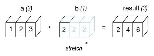
The term broadcasting describes how NumPy treats arrays with different shapes during arithmetic operations. Subject to certain constraints, the smaller array is “broadcast” (strechted) across the larger array so that they have compatible shapes.
a = np.array([1.0, 2.0, 3.0])
b = 2.0
a * b
array([2., 4., 6.])
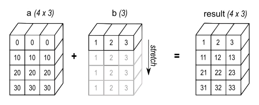
a = np.ones((4,3))
b = np.arange(3)
c = a + b; c.shape
(4, 3)
Another example: adding a column array (3, 1) and a row array (3) results in an array of shape (3, 3).
a = np.ones((3,1)); a
array([[1.],
       [1.],
       [1.]])
b = np.arange(3); b
array([0, 1, 2])
c = a + b; c.shape
(3, 3)
c
array([[1., 2., 3.],
       [1., 2., 3.],
       [1., 2., 3.]])
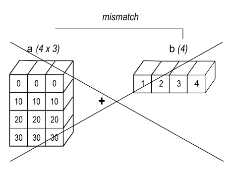
When the trailing dimensions of the arrays are unequal, broadcasting fails because it is impossible to align the values in the rows of the 1st array with the elements of the 2nd arrays for element-by-element addition.
The following rules apply when broadcasting:
Rule 1: If the two arrays differ in their number of dimensions, the shape of the one with fewer dimensions is padded with ones on its leading (left) side.
Rule 2: If the shape of the two arrays does not match in any dimension, the array with shape equal to 1 in that dimension is stretched to match the other shape.
Rule 3: If in any dimension the sizes disagree and neither is equal to 1, an error is raised.
You can also directly broadcast and stretch an array to a new shape with np.broadcast_to(). Change the output dimensions and see what happens.
a = np.arange(3)
np.broadcast_to(a, (2, 4, 3))
array([[[0, 1, 2],
        [0, 1, 2],
        [0, 1, 2],
        [0, 1, 2]],

       [[0, 1, 2],
        [0, 1, 2],
        [0, 1, 2],
        [0, 1, 2]]])
Masking#
Masking replaces elements of an array based on boolean operations, i.e., comparisons like > (greater), < (less than), == (equal), != (not equal). For example, the code below creates a boolean mask m and replace all masked values in x with the number 2.
x = np.arange(5)
x
array([0, 1, 2, 3, 4])
m = x > 2
m
array([False, False, False, True, True])
x[m] = 2
x
array([0, 1, 2, 2, 2])
Searching#
Searching functions return the indices of array elements, e.g., of the maximum (minimum) values along an axis with np.argmax() (np.argmin()). Their NaN-ignoring counterparts are np.nanargmax() and np.nanargin(). The functions np.nonzereo() and np.argwhere() return the indices of the non-zero elements.
np.random.seed(42) # fixes the random number generator
a = np.random.randint(100, size=18).reshape(3,2,3);  a
array([[[51, 92, 14],
        [71, 60, 20]],

       [[82, 86, 74],
        [74, 87, 99]],

       [[23,  2, 21],
        [52,  1, 87]]])
np.argmax(a, axis=2) # change the axis keyword to change the dimension
array([[1, 0],
       [1, 2],
       [0, 2]])
We can also search indices along a certain axis and then grab the corresponding values. Below, we first search for the maximum values along axis 0. Then we use take_along_axis() to grab those values from the array.
j = np.argmax(a, axis=0); j
array([[1, 0, 1],
       [1, 1, 1]])
xtract = np.take_along_axis(a, j[np.newaxis, :, :], axis=0)
xtract.shape
(1, 2, 3)
Note, we need to add a band-dimension to j to match the three dimensions of a. The result then contains a trailing dimension of length 1. We can remove that trailing dimension and covert the result to a two-dimensional array using np.squeeze() (see section Changing dimensions).
xtract.squeeze()
array([[82, 92, 74],
       [74, 87, 99]])
Fancy indexing#
…extends the simple indexing with arrays of indices instead of scalars. The result may surprise you. With fancy indexing, the shape of the result reflects the shape of the index arrays rather than the shape of the array being indexed:
X = np.arange(12).reshape((3, 4))
X
array([[ 0,  1,  2,  3],
       [ 4,  5,  6,  7],
       [ 8,  9, 10, 11]])
row = np.array([ 0 , 1 , 2 ])
col = np.array([ 2 , 1 , 3 ])
X[row,col]
array([ 2, 5, 11])