Introduction to GEE#
Background#
So far in this course, we have covered the use of python in handling geodata. Specifically, we have learned how to manage (large) raster and vector data and we got in contact with a large variety of tools and techniques. What all these had in common, was that usually you were provided with some kind of data, prepared by us. In addition, so far there was always enough computing power and disc space available for you. However, in your own research or in work you do outside of the university you will likely face the issue that you want to work with large data, but (a) won’t have the infrastructure to process them, and (b) may face restrictions because you want to access data as a private person. This is, why we want to expose you during the next few weeks to Google Earth Engine (GEE) as a huge data and processing engine, that you can use for your own work. GEE is around since ~2012 and it received a lot of attention with the publication by Hansen et al. (2013) in Science. Since then, the number of studies using GEE has exploded and the data catalogue seems to be growing day after day.
There are a lot of different tutorials and packages that help you doing some sort of analysis. Many of them use the language JavaScript , which GEE was initially prepared for, but increasingly you find tutorials and tools that use Python as an API. What these tools and tutorials all have in common is that they help you running some analysis in GEE and visualize the results. This can include time series analyses, image classifications, or simply the visualization of datasets (which there are a lot in GEE). They are designed to visualize the results directly in the browser, and, as we will learn, compute the results on-the-fly when zooming in/out or moving to a different place on the Earth. This is all pretty fantastic, and - as already said - there are a lot of tutorials out there, many of which we will provide links to. Though, GEE also has a number of limitations, such as a limited amount of algorithms implemented that can be applied. While for example in case of “simple” classifications this is not too big of a problem, in our daily research we often want to do more, for example designing new methods and tools that use image classifications or regressions as input. In the majority of these cases, GEE does not have the capabilities to flexibly implement and test new analysis methods. Thus, at some point in our analysis we need to export large amounts of pre-processed data from GEE to our own drives and work on them further. Here is, where it becomes tricky as GEE has mechnisms in its architecture that prevents exports of large data at once.
This part of the course therefore will not provide yet another tutorial of doing image classifications in GEE, but we want to continue with the general research line of large-scale processing. Specifically, we want to teach you in these sessions on how to use GEE as a large pre-processing-engine from which you export intermediate results to your own computer. Focussing on this part, will in our eyes nicely complement existing tutorials, which we will provide links to.

Fig. 4 Overview about the different components, that GEE offers. The figure is derived from the GEE-website).#
We will focus on the first two elements (from the left) and we will use python as our API. In short, what GEE provides to us, is:
An extensive archive of data, including many complete satellite image archives (e.g., Landsat, Sentinel-1/2, MODIS, Planet-NICFI mosaics) as well as land-cover products (e.g., global forest watch, ESA World-Cover) both at the global and national (primarily United States) scale.
Simple (e.g., linear regression, random forests) & more advanced processing algorithms, particularly in the satellite image domain (e.g., LandTrendr, CCDC)
Nearly unlimited computing power
On the opposite, what it does not provide to us:
advanced processing solutions, particularly with respect to remote sensing data processing (e.g., FORCE); but also a higher diversity of classification and rgression algorithm (e.g., gradient boosting regression)
Although GEE provides some detail on how it handles data and applies algorithms, for many instances it remains a “black box”.
Nice cartography (although this is getting better)
DIY-parallelization (“The price of liberation from these details is that the user is unable to influence them.” (Gorelick, et al. 2017))
Easy extrapolation across large geographic spaces and export/download of these processing results
Having these elements in mind, what we want to do in this course, is:
to advertise GEE as a great source to do large area processing (but not necessarily only)
Show its power, but also its limitations and develop ways to work around this
Motivate you to use the best of the two worlds: (1) Data archives and processing power in GEE, (2) Advanced functionality of local python processing and use of gdal and osr
There are many important aspects with regards to GEE that you will probably learn if you keep using it. Though, one fundamental principle is important for our understanding: the distinction between server- and client-side operations. In general, we have a client side library that will be translated into complex geospatial analyses into EE requests:
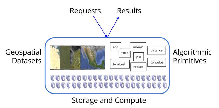
Fig. 5 Schematic representation about the differentiation between server-side and client-side operations (Source: https://geohackweek.github.io/GoogleEarthEngine/).#
This is an important aspect, as we will have to always think about what a certain operation is done locally on your computer, and what operation we want GEE to do. In other words, on the client-side (i.e., our computers) we create and manipulate “proxy objects”, which do not contain any data, but are just handles for objects on the server-side. This is really important to consider, because it means that, compared to the processes we have been thinking so far, we hardly can create/modify variables step-by-step.
Client library#
The client library lets you run processing tasks on the Google servers. The library can be accessed via a JavaScript and Python API (Application Interface). To better understand the API, check out the documentation. Below is a list of some examples.
Client Libraries:
ee.Algorithms
ee.Array
ee.Blob
ee.Classifier
ee.Image
ee.ImageCollection
ee.Reducer
Some libraries such as ee.Algorithms and ee.Reducer contain functions that are applied to other EE objects. They work like a collection of tools. You can access them as follows:
ee.Algorithms.HillShadow(image, azimuth, zenith, neighborhoodSize, hysteresis)
Other libraries correspond to EE data types that have their own functions (methods), e.g., ee.Dictionary, ee.Image.
Data types#
There are many good GEE tutorials online, including this one. We do not want to re-invent those tutorials and possibly create a terrible new version of it. Instead, we want to focus on doing these types of analyses and extract the data to our own drive - both for individual locations but also across large geographic extents. Here, we briefly introduce the basic elements of geographic features that we will work with in the context of the course. For a more complete overview of Earth Engine’s data types see here. When we introduce the data types, we will also use some visualization tools, specifically from the geemap library. This package has become quite popular in the last years. The author/developer is Quisheng Wu, a professor at the University of Tenessee. Originally being a thematic expert in Wetland mapping, he has become an important developer for GEE using python. The strength of his tool is that it brings together the functionality of QGIS in a ipynb. Many tools and tricks for visualization are available through his package, and we really recommend checking it out. For example, the package allows to download TimeLapse videos (see some examples for what a TimeLaps is here) and also some image composites and image classifications. The package also builds on different visualization backends, all of which have a different functionality. You can find out more about this here. The weakness of the tool/library is that it is not perfect if we want to extract large amounts of data from GEE or do complex operations as the package of course also faces memory and computation restrictions from the side of GEE. So, for our course, it is mostly suitable for visualizing data. The rest - as you have learned during the past weeks of the course - will have to be implemented manually.
We start by importing the package and by authenticating our computer with google. This basically creates a connection between you and your computer and stores the connection details in something similar to a cookie. This is done by the code line ee.Authenticate() and has only be execute once. What you need to do, however, every time you start working is to instantiate a GEE session via ee.Initialize(). Below is a good code chunk that you can possibly use as a standard chunk inside your scripts.
import ee
import geemap.foliumap as geemap
try:
    ee.Initialize()
except Exception as e:
    ee.Authenticate()
    ee.Initialize()
Vector data#
Contrary to the previous parts of this book, we will start with introducing vector data, primarily because we will use them to make some spatial selections later on with raster data. In GEE vector data are considered as features. A feature consists of a Geometry and a dictionary of properties (comparable to attributes). Below you find an example for how to build geometries and correspoinding features:
point_geom = ee.Geometry.Point([-60, -20])
rectangle_geom = ee.Geometry.Rectangle([-60, -20, -62, -22])
polygon_geom = ee.Geometry.Polygon([[[-60, -20], [-62, -20], [-62, -22], [-60, -22], [-60, -20]]])
point_feat = ee.Feature(point_geom, {'ID': 1})
rectangle_feat = ee.Feature(rectangle_geom, {'ID': 2})
polygon_feat = ee.Feature(polygon_geom, {'ID': 3})
Many features combined result in a ee.FeatureCollection(), which corresponds to what we have got to know as a layer in general vector data. An ee.FeatureCollection() is build through a list of features. While it is in principle possible to combined different types of features/geometries (e.g., points and polygons), we generally recommend to keep these separate for data sanity. Keep in mind, that these are only container objects, which are only created server-side. How we retrieve these objects, we show in the next chapter.
# Build a second point feature
point_geom_2 = ee.Geometry.Point([-61, -21])
point_feat_2 = ee.Feature(point_geom_2, {'ID': 2})
# Create a feature collection from the point features
fc = ee.FeatureCollection([point_feat, point_feat_2])
fc
- type:FeatureCollection
- ID:Integer
- system:index:String
- type:Feature
- id:0
- type:Point
- 0:-60
- 1:-20
- ID:1
- type:Feature
- id:1
- type:Point
- 0:-61
- 1:-21
- ID:2
Besides manually created feature collections, there are many different datasets stored in GEE. What we have learned in our section on vector selections is that vector data can be either selected by location or by attribute. In GEE we do this trough applying a filter to a ee.FeatureCollection(), which corresponds to the .SetAttributeFilter() method we learned before. Below you find an example, that loads the FAO country borders from GEE (i.e., an ee.FeatureCollection())`, and then selects the country Germany. We then use geemap to visualize the feature on a map.
fao = ee.FeatureCollection("FAO/GAUL/2015/level0")
ger = fao.filter(ee.Filter.eq('ADM0_NAME', 'Germany')) # Filter by country name
- type:FeatureCollection
- id:FAO/GAUL/2015/level0
- version:1701682497889631
- ADM0_CODE:Integer
- ADM0_NAME:String
- DISP_AREA:String
- EXP0_YEAR:Integer
- STATUS:String
- STR0_YEAR:Integer
- Shape_Area:Float
- Shape_Leng:Float
- system:index:String
- system:asset_size:139687468
- type:Feature
- id:00000000000000000018
- type:GeometryCollection
- type:LineString
- 0:6.507085903474608
- 1:49.79082178209467
- 0:6.507081444373555
- 1:49.79082178209467
- type:Polygon
- 0:13.117172607224203
- 1:54.54923997306883
- 0:13.11768983373403
- 1:54.54152126201734
- 0:13.125711799638934
- 1:54.544375109446136
- 0:13.125292545141015
- 1:54.54944063669055
- 0:13.117172607224203
- 1:54.54923997306883
- type:Polygon
- 0:11.488378934126983
- 1:54.02471149233134
- 0:11.498108708616023
- 1:54.02302594201704
- 0:11.502465156548519
- 1:54.03002669387053
- 0:11.497279245852585
- 1:54.032073455369
- 0:11.488378934126983
- 1:54.02471149233134
- type:Polygon
- 0:8.723959251499942
- 1:54.47121015151016
- 0:8.724637034054945
- 1:54.46891821696516
- 0:8.728489628879732
- 1:54.46748238483795
- 0:8.74907727756338
- 1:54.47241414869194
- 0:8.735392288338751
- 1:54.47286002367312
- 0:8.723959251499942
- 1:54.47121015151016
- type:Polygon
- 0:8.548168084077075
- 1:54.47179875635074
- 0:8.553724099368372
- 1:54.464178161823
- 0:8.55759906360996
- 1:54.46321055706897
- 0:8.568385645993853
- 1:54.468307330171456
- 0:8.5560339016057
- 1:54.47259700499605
- 0:8.548168084077075
- 1:54.47179875635074
- type:Polygon
- 0:9.226361622198484
- 1:53.8728122221724
- 0:9.248848892550042
- 1:53.866707681071745
- 0:9.255501861158027
- 1:53.86817029400413
- 0:9.253330279921919
- 1:53.8707298187551
- 0:9.227583423362466
- 1:53.874181114484614
- 0:9.226361622198484
- 1:53.8728122221724
- type:Polygon
- 0:13.157857431394602
- 1:54.51224732293273
- 0:13.158664485536162
- 1:54.507159467853405
- 0:13.162829372599784
- 1:54.50350747744556
- 0:13.165665340596707
- 1:54.50405142300959
- 0:13.169714156658353
- 1:54.50834554430214
- 0:13.164430105246515
- 1:54.51327730515157
- 0:13.157857431394602
- 1:54.51224732293273
- type:Polygon
- 0:13.769993884716941
- 1:54.207169004007135
- 0:13.772410725982782
- 1:54.19096906228723
- 0:13.77503269899532
- 1:54.192654633990685
- 0:13.774742803476508
- 1:54.20276786622938
- 0:13.778586545419458
- 1:54.20713774993613
- 0:13.774078418062238
- 1:54.21060691556489
- 0:13.769993884716941
- 1:54.207169004007135
- type:Polygon
- 0:13.112717946605157
- 1:54.30978625888415
- 0:13.118782273409469
- 1:54.30426141225796
- 0:13.123865698161293
- 1:54.30423023116544
- 0:13.129662464975066
- 1:54.308974695076714
- 0:13.12225146578916
- 1:54.314401457616306
- 0:13.1143143102151
- 1:54.313661188347886
- 0:13.112717946605157
- 1:54.30978625888415
- type:Polygon
- 0:8.703193141092813
- 1:54.16790660997541
- 0:8.703763932957314
- 1:54.163327132326096
- 0:8.708753689808903
- 1:54.16187791194964
- 0:8.716160286511016
- 1:54.1709031209473
- 0:8.714287367443092
- 1:54.172530673354885
- 0:8.70766118144869
- 1:54.17217838462211
- 0:8.703193141092813
- 1:54.16790660997541
- type:Polygon
- 0:9.507311764977857
- 1:53.703665103716105
- 0:9.52858611317405
- 1:53.669116003165996
- 0:9.532099955400787
- 1:53.66995428560701
- 0:9.531016357848364
- 1:53.68918639799358
- 0:9.52672225073185
- 1:53.69431439948739
- 0:9.509746490976825
- 1:53.70566725849446
- 0:9.507311764977857
- 1:53.703665103716105
- type:Polygon
- 0:9.579183538811026
- 1:53.6014179588937
- 0:9.59354635297988
- 1:53.59172834601765
- 0:9.607418614737192
- 1:53.587041789742656
- 0:9.60987998546169
- 1:53.589498761434236
- 0:9.595173892319476
- 1:53.59944701035905
- 0:9.580124416162064
- 1:53.604137985159916
- 0:9.579183538811026
- 1:53.6014179588937
- type:Polygon
- 0:13.91301069172125
- 1:54.24189199286937
- 0:13.916809805222533
- 1:54.24121418070031
- 0:13.923226421432023
- 1:54.246810366935904
- 0:13.928104671713559
- 1:54.2479029022187
- 0:13.92817608177695
- 1:54.250654093419236
- 0:13.92282951616981
- 1:54.25142106000116
- 0:13.913273786497605
- 1:54.245775879001066
- 0:13.91301069172125
- 1:54.24189199286937
- type:Polygon
- 0:12.720883380374884
- 1:54.40811838128173
- 0:12.725690238665077
- 1:54.40605376996563
- 0:12.734390002522204
- 1:54.4065532096773
- 0:12.741783176899721
- 1:54.408947742863056
- 0:12.741622619295635
- 1:54.41301889628229
- 0:12.733721104939862
- 1:54.41432986252021
- 0:12.726608802482371
- 1:54.413496047959185
- 0:12.720883380374884
- 1:54.40811838128173
- type:Polygon
- 0:13.39805585468481
- 1:54.17975438952989
- 0:13.406175804338568
- 1:54.16922650165039
- 0:13.412900172569909
- 1:54.16820537844359
- 0:13.417417160157324
- 1:54.15959925890235
- 0:13.420774889991634
- 1:54.16523114779644
- 0:13.424966517085133
- 1:54.16706827985161
- 0:13.415366035195667
- 1:54.17561190946272
- 0:13.39805585468481
- 1:54.17975438952989
- type:Polygon
- 0:12.679846224809582
- 1:54.42038982427296
- 0:12.684920764336685
- 1:54.417397768802594
- 0:12.714426611785484
- 1:54.420800047909395
- 0:12.729596447699773
- 1:54.41709454593211
- 0:12.734447958718485
- 1:54.4197700217897
- 0:12.73335991242551
- 1:54.42357810403695
- 0:12.713088799683666
- 1:54.4287640250298
- 0:12.698494166084298
- 1:54.430726047658695
- 0:12.679846224809582
- 1:54.42038982427296
- type:Polygon
- 0:8.681080503652378
- 1:54.133977284500595
- 0:8.685098099634585
- 1:54.128202733786
- 0:8.695862429222492
- 1:54.125745786444284
- 0:8.696343989396233
- 1:54.12779697681108
- 0:8.691809074903691
- 1:54.13061064167957
- 0:8.691550452226771
- 1:54.13358490058828
- 0:8.697949267589848
- 1:54.137598078702595
- 0:8.685102638913111
- 1:54.1371120707609
- 0:8.681080503652378
- 1:54.133977284500595
- type:Polygon
- 0:6.855925806139272
- 1:53.5954917792516
- 0:6.858222229777362
- 1:53.59411841718147
- 0:6.865517317211963
- 1:53.59754295098604
- 0:6.871648636046202
- 1:53.59662440303444
- 0:6.874725372507594
- 1:53.60073568956811
- 0:6.873195931958492
- 1:53.60325059658798
- 0:6.869361094897876
- 1:53.603937366940094
- 0:6.857464232519264
- 1:53.60006234817717
- 0:6.855925806139272
- 1:53.5954917792516
- type:Polygon
- 0:12.927098894099904
- 1:54.43724966830102
- 0:12.930242548351702
- 1:54.434574210388064
- 0:12.935054015352328
- 1:54.43524756852408
- 0:12.942830669865112
- 1:54.44013467242679
- 0:12.949265128444512
- 1:54.44118707399727
- 0:12.963587762532633
- 1:54.43978687744719
- 0:12.962490862560996
- 1:54.44305541773764
- 0:12.947356673920233
- 1:54.44426382299459
- 0:12.930135564915451
- 1:54.44191391668933
- 0:12.927098894099904
- 1:54.43724966830102
- type:Polygon
- 0:8.486427406633844
- 1:53.918397592644915
- 0:8.492424826829192
- 1:53.91495960625007
- 0:8.501713174054526
- 1:53.91406783120022
- 0:8.509842113256004
- 1:53.91440670834566
- 0:8.518902984985134
- 1:53.91862052845444
- 0:8.519455862308172
- 1:53.92272737727994
- 0:8.5051198731933
- 1:53.93161440641063
- 0:8.49747258881941
- 1:53.933777032000314
- 0:8.489535385602519
- 1:53.92863570567691
- 0:8.486427406633844
- 1:53.918397592644915
- type:Polygon
- 0:8.713520399728216
- 1:54.63765953165679
- 0:8.72080660948247
- 1:54.63366864730688
- 0:8.727432845662877
- 1:54.63242003508399
- 0:8.735031182547619
- 1:54.635269420679975
- 0:8.742428754801486
- 1:54.64223453670113
- 0:8.737969693016382
- 1:54.64778614388576
- 0:8.732444847582414
- 1:54.64741606265491
- 0:8.727593389967458
- 1:54.64452208932281
- 0:8.71854591407788
- 1:54.644437367149294
- 0:8.714028821002588
- 1:54.640165502146594
- 0:8.713520399728216
- 1:54.63765953165679
- type:Polygon
- 0:8.795367229600945
- 1:54.556646564782675
- 0:8.79764144292452
- 1:54.55501010254736
- 0:8.812864713897788
- 1:54.55338692835151
- 0:8.8236245969896
- 1:54.54864248489578
- 0:8.82831550273101
- 1:54.5483348315132
- 0:8.835093379143608
- 1:54.55050634453775
- 0:8.840934839362184
- 1:54.55772121816439
- 0:8.83079479484985
- 1:54.55903216321526
- 0:8.823669175435318
- 1:54.557779185339776
- 0:8.812454534366836
- 1:54.56115917556565
- 0:8.795367229600945
- 1:54.556646564782675
- type:Polygon
- 0:13.518843910052407
- 1:54.316243058281565
- 0:13.523419022320063
- 1:54.31219867674698
- 0:13.527053199370146
- 1:54.31048189205924
- 0:13.531043977437893
- 1:54.31939560948686
- 0:13.539248860483879
- 1:54.323948405692875
- 0:13.548786795976774
- 1:54.324804526017566
- 0:13.545348849753994
- 1:54.330266951071025
- 0:13.546597412074435
- 1:54.33317872065791
- 0:13.542677835709176
- 1:54.33316530559289
- 0:13.531806508709765
- 1:54.326418726874344
- 0:13.525059915288073
- 1:54.31857516583356
- 0:13.518843910052407
- 1:54.316243058281565
- type:Polygon
- 0:8.439736061870514
- 1:54.57288661313248
- 0:8.44340148152195
- 1:54.566215794206634
- 0:8.449541649541374
- 1:54.56270651027379
- 0:8.457768704051755
- 1:54.56236758650443
- 0:8.457626009123997
- 1:54.56876193880859
- 0:8.463949028177717
- 1:54.56981873561417
- 0:8.455650629054189
- 1:54.57838470215257
- 0:8.45662712361825
- 1:54.58316480791149
- 0:8.455503461321637
- 1:54.584551603990356
- 0:8.44564885836247
- 1:54.58354383320956
- 0:8.44077065575726
- 1:54.579267553295985
- 0:8.439736061870514
- 1:54.57288661313248
- type:Polygon
- 0:9.674220340598788
- 1:53.5647908697032
- 0:9.698549247906863
- 1:53.5613261811744
- 0:9.729198841560718
- 1:53.558064356406454
- 0:9.759848483458075
- 1:53.5548025300148
- 0:9.776423034640242
- 1:53.55599755803265
- 0:9.784685696005274
- 1:53.55350046431825
- 0:9.787829409909769
- 1:53.554570590739516
- 0:9.784221941348683
- 1:53.55786142276009
- 0:9.771379766041704
- 1:53.56069298886545
- 0:9.740620916591407
- 1:53.5596183328382
- 0:9.698477892470217
- 1:53.56465265746594
- 0:9.675116653942743
- 1:53.567983575323254
- 0:9.674220340598788
- 1:53.5647908697032
- type:Polygon
- 0:7.367799372065748
- 1:53.72929603869703
- 0:7.3746887001748895
- 1:53.726749914934935
- 0:7.410780725067316
- 1:53.721996471075165
- 0:7.429245884747157
- 1:53.72212578575427
- 0:7.434280160799556
- 1:53.72415019460851
- 0:7.439640043856382
- 1:53.722750091817844
- 0:7.440451558211103
- 1:53.72549243818712
- 0:7.43095810892545
- 1:53.73376852392734
- 0:7.416733645126565
- 1:53.73453102734467
- 0:7.396796959621463
- 1:53.739663444551994
- 0:7.389871929066808
- 1:53.73947172861039
- 0:7.377515858323724
- 1:53.733599078952686
- 0:7.367799372065748
- 1:53.72929603869703
- type:Polygon
- 0:8.451512636790072
- 1:54.54303740295375
- 0:8.454839071762986
- 1:54.52792099143215
- 0:8.46051110905846
- 1:54.51276900753087
- 0:8.46831894287411
- 1:54.50215190781116
- 0:8.483921350182703
- 1:54.50034147443036
- 0:8.490645649440385
- 1:54.5018442276862
- 0:8.485334843846944
- 1:54.506258740415646
- 0:8.48443411892769
- 1:54.51312127203227
- 0:8.477946182903644
- 1:54.51755358682578
- 0:8.482534550377371
- 1:54.5341637853071
- 0:8.480407563699131
- 1:54.53990263052532
- 0:8.471467020076517
- 1:54.54185123708476
- 0:8.466325695133705
- 1:54.5506000631775
- 0:8.457322799843
- 1:54.551179728781435
- 0:8.45369752478092
- 1:54.54871825337404
- 0:8.451512636790072
- 1:54.54303740295375
- type:Polygon
- 0:7.853208240660829
- 1:53.78671587829644
- 0:7.856958380225949
- 1:53.782568876304325
- 0:7.869475027455545
- 1:53.774689653800834
- 0:7.874179440035716
- 1:53.778074108976284
- 0:7.871249746422619
- 1:53.784040445203544
- 0:7.8771224508918865
- 1:53.787870819528365
- 0:7.881380835578291
- 1:53.78852184251272
- 0:7.900572774685516
- 1:53.78582850740874
- 0:7.920076924136115
- 1:53.78039290057363
- 0:7.945529520757621
- 1:53.78151655557745
- 0:7.969309837978944
- 1:53.775991725566904
- 0:7.976894763760266
- 1:53.77889014660957
- 0:7.950169161251922
- 1:53.7849946712733
- 0:7.923443563292369
- 1:53.791099175907426
- 0:7.878415581423954
- 1:53.793346533387485
- 0:7.855018646895009
- 1:53.788107150230154
- 0:7.853208240660829
- 1:53.78671587829644
- type:Polygon
- 0:12.975943911415676
- 1:54.44375550294351
- 0:12.976028616063587
- 1:54.44308221801881
- 0:12.977049851041013
- 1:54.43522079135961
- 0:12.990534156126788
- 1:54.43614830160541
- 0:13.008102957398904
- 1:54.443519134667454
- 0:13.018474769627506
- 1:54.44460270933544
- 0:13.030264690300378
- 1:54.44469639706857
- 0:13.034960065773824
- 1:54.441940624952956
- 0:13.039994503737198
- 1:54.441454612835265
- 0:13.060760540010639
- 1:54.454386009654385
- 0:13.0592845546701
- 1:54.45767235232361
- 0:13.051347306412717
- 1:54.46243022040296
- 0:13.04896618713293
- 1:54.45429678025402
- 0:13.045238405247582
- 1:54.450359398695134
- 0:13.03583852065508
- 1:54.447857866644846
- 0:13.00572181253131
- 1:54.448682824331506
- 0:12.99695522809757
- 1:54.44247571299496
- 0:12.975943911415676
- 1:54.44375550294351
- type:Polygon
- 0:8.663953118872078
- 1:54.062488970758
- 0:8.665977479882532
- 1:54.05560415441378
- 0:8.676701653642995
- 1:54.04378309351683
- 0:8.682779422033345
- 1:54.04094707493594
- 0:8.691675371618427
- 1:54.04058145205158
- 0:8.695746470381152
- 1:54.04485768007825
- 0:8.688821511634307
- 1:54.05479260954271
- 0:8.697030717808968
- 1:54.05626406150112
- 0:8.699853355548065
- 1:54.058729965607284
- 0:8.69798938777054
- 1:54.06036198339426
- 0:8.689847071355661
- 1:54.06049134361633
- 0:8.685713493868953
- 1:54.072209783145
- 0:8.688286423818804
- 1:54.07764990846025
- 0:8.69588468750791
- 1:54.08279127727862
- 0:8.69132308587235
- 1:54.08491383160911
- 0:8.675181094949805
- 1:54.07968330591202
- 0:8.665906178933675
- 1:54.071603410325416
- 0:8.663953118872078
- 1:54.062488970758
- type:Polygon
- 0:8.508758500382307
- 1:54.58107796000469
- 0:8.510988107965442
- 1:54.57807700346573
- 0:8.51986175289794
- 1:54.57430016566913
- 0:8.538130626301786
- 1:54.569930213723254
- 0:8.547601779169236
- 1:54.56179680360654
- 0:8.568791424168236
- 1:54.56172544747362
- 0:8.575966105297574
- 1:54.56436076854691
- 0:8.578088636228678
- 1:54.56821350836715
- 0:8.575899199080554
- 1:54.57212855322675
- 0:8.570133613736024
- 1:54.574951201347396
- 0:8.562031443269603
- 1:54.58318714082625
- 0:8.561473996917645
- 1:54.583753434834755
- 0:8.55369291227829
- 1:54.58546574571464
- 0:8.549737691857478
- 1:54.58472104167191
- 0:8.53905361028867
- 1:54.582705555006214
- 0:8.528833420788581
- 1:54.58239337546284
- 0:8.517190649503103
- 1:54.585755580335444
- 0:8.509681578140624
- 1:54.58449363668101
- 0:8.508758500382307
- 1:54.58107796000469
- type:Polygon
- 0:6.871367734530923
- 1:53.64917937151915
- 0:6.872491389391374
- 1:53.63546759446936
- 0:6.875938253882135
- 1:53.63157929123077
- 0:6.8843749095561435
- 1:53.62814128827223
- 0:6.898956121026164
- 1:53.62561301378175
- 0:6.904712819590744
- 1:53.62606341038447
- 0:6.900886911821124
- 1:53.63087028964933
- 0:6.903196770490714
- 1:53.63338074578797
- 0:6.908565495156502
- 1:53.63108876081858
- 0:6.913189638898416
- 1:53.63771055920455
- 0:6.928577989755125
- 1:53.64682942683706
- 0:6.9262771106670815
- 1:53.64911695654448
- 0:6.918602973429988
- 1:53.65049921940438
- 0:6.910536494878109
- 1:53.64913920171222
- 0:6.895576163321852
- 1:53.65623813220477
- 0:6.888664566781891
- 1:53.65647445422881
- 0:6.883665855662749
- 1:53.65488255556139
- 0:6.87866724007139
- 1:53.65008457325175
- 0:6.871367734530923
- 1:53.64917937151915
- type:Polygon
- 0:13.120788966918278
- 1:54.44863824732282
- 0:13.124017372794516
- 1:54.44406320037905
- 0:13.137046793364016
- 1:54.444540263462386
- 0:13.145808990844525
- 1:54.44792031442623
- 0:13.173963637576861
- 1:54.45876705000574
- 0:13.202118392729009
- 1:54.469613796696905
- 0:13.215727649975523
- 1:54.468681847870954
- 0:13.218362917906134
- 1:54.46533754993949
- 0:13.224913365712048
- 1:54.46705873414898
- 0:13.227972300157488
- 1:54.47423347082993
- 0:13.223406233138519
- 1:54.48295546414521
- 0:13.22855198224681
- 1:54.48585389162445
- 0:13.226697075794158
- 1:54.48692849868885
- 0:13.208084727599307
- 1:54.485586343144014
- 0:13.198033891280573
- 1:54.489314116336224
- 0:13.200044989209568
- 1:54.49219021328227
- 0:13.19712879168952
- 1:54.493715295048915
- 0:13.181169661199784
- 1:54.49477207853548
- 0:13.156368068367854
- 1:54.489042163335114
- 0:13.127134223537988
- 1:54.46941318110776
- 0:13.120788966918278
- 1:54.44863824732282
- type:Polygon
- 0:8.437693865168999
- 1:54.45026133352793
- 0:8.439089516943627
- 1:54.44590482089946
- 0:8.461313715196969
- 1:54.433954372996645
- 0:8.466949994600899
- 1:54.42816652112459
- 0:8.478160195014588
- 1:54.42481325695896
- 0:8.479150059224736
- 1:54.42478203056829
- 0:8.490663544864764
- 1:54.42441192859993
- 0:8.49390526846822
- 1:54.42733261247493
- 0:8.493312221849163
- 1:54.431912128879205
- 0:8.500865973995351
- 1:54.43500675227573
- 0:8.503724234217929
- 1:54.43793636301105
- 0:8.501516891360257
- 1:54.441392170813316
- 0:8.491987893605803
- 1:54.447692920282016
- 0:8.49065453212557
- 1:54.45342282702209
- 0:8.477843585836062
- 1:54.456111709731026
- 0:8.474450261830219
- 1:54.45935347077147
- 0:8.47701865998144
- 1:54.46480244712059
- 0:8.475569391449934
- 1:54.4677944968805
- 0:8.46055561904385
- 1:54.46434316513539
- 0:8.444502915479907
- 1:54.46433428835983
- 0:8.44128784433046
- 1:54.46209132451864
- 0:8.437693865168999
- 1:54.45026133352793
- type:Polygon
- 0:7.671540033025189
- 1:53.757580090615434
- 0:7.675446188685789
- 1:53.755729600970824
- 0:7.67840252510312
- 1:53.754329413874665
- 0:7.689938215835399
- 1:53.75355801800385
- 0:7.690772165232274
- 1:53.75675071918482
- 0:7.6986067669941916
- 1:53.76308707169922
- 0:7.714762090219616
- 1:53.76227996428413
- 0:7.722792924656585
- 1:53.759702622868275
- 0:7.754729059792753
- 1:53.75898922290562
- 0:7.765256932041455
- 1:53.76484847981057
- 0:7.792751760071413
- 1:53.771474658222694
- 0:7.807792263063216
- 1:53.77225949770993
- 0:7.812055211373751
- 1:53.77336529807726
- 0:7.8140439022984545
- 1:53.77609427903925
- 0:7.811011774026645
- 1:53.77817666119626
- 0:7.770616769940035
- 1:53.78034381457842
- 0:7.750171796231803
- 1:53.778907960263275
- 0:7.748883127311083
- 1:53.77892133801421
- 0:7.699721558733127
- 1:53.77930487936781
- 0:7.694308232703851
- 1:53.77843090504311
- 0:7.678786027123259
- 1:53.76969102427692
- 0:7.671540033025189
- 1:53.757580090615434
- type:Polygon
- 0:8.119973986495838
- 1:53.71709590934986
- 0:8.121463357436298
- 1:53.71547731025522
- 0:8.12952535351205
- 1:53.71493329163723
- 0:8.136151533578596
- 1:53.717827228557205
- 0:8.142568205776
- 1:53.71387204566834
- 0:8.151004854059057
- 1:53.71308718802538
- 0:8.155330169822136
- 1:53.71601241314289
- 0:8.153872064308239
- 1:53.71854065082698
- 0:8.161211738516016
- 1:53.71960194836647
- 0:8.165996323203665
- 1:53.72480125183583
- 0:8.172983769730152
- 1:53.726776671614495
- 0:8.185268520486048
- 1:53.72594721290215
- 0:8.192238162318587
- 1:53.727240409621935
- 0:8.193455510622163
- 1:53.729282654681064
- 0:8.188189245346305
- 1:53.73300155995853
- 0:8.16332085444497
- 1:53.73739822757308
- 0:8.141341984750024
- 1:53.73605155538631
- 0:8.12412534083353
- 1:53.726874718809555
- 0:8.122912469518543
- 1:53.72505989778524
- 0:8.12863797445016
- 1:53.72362407847203
- 0:8.127799729904146
- 1:53.72134992192033
- 0:8.12164609871955
- 1:53.7214168346163
- 0:8.119973986495838
- 1:53.71709590934986
- type:Polygon
- 0:7.471023144100423
- 1:53.73673825509712
- 0:7.471250542865789
- 1:53.72691483782245
- 0:7.478474317159936
- 1:53.72139003408082
- 0:7.483107279718418
- 1:53.72273222174236
- 0:7.48895318113482
- 1:53.727267166318235
- 0:7.496997365933463
- 1:53.72648233517703
- 0:7.498937179882185
- 1:53.72629506927517
- 0:7.505951270568266
- 1:53.73150771541799
- 0:7.50532259499888
- 1:53.73996661945513
- 0:7.514249651026192
- 1:53.74447923364811
- 0:7.533098288692514
- 1:53.743908496093226
- 0:7.568592699337558
- 1:53.74870649702099
- 0:7.592270607999191
- 1:53.74816250520278
- 0:7.620871294731315
- 1:53.745380003096614
- 0:7.628884287075774
- 1:53.74189298986173
- 0:7.632357943238176
- 1:53.74233001832637
- 0:7.6344403057732295
- 1:53.75030728005579
- 0:7.632946472721029
- 1:53.75260377247618
- 0:7.61338893855667
- 1:53.756625894377784
- 0:7.571080881362861
- 1:53.758743906236575
- 0:7.532951135753853
- 1:53.75772725729057
- 0:7.494821378717351
- 1:53.75671055629123
- 0:7.483678037975885
- 1:53.75382105079861
- 0:7.4773729271800295
- 1:53.74904089728216
- 0:7.471023144100423
- 1:53.73673825509712
- type:Polygon
- 0:7.142583568498894
- 1:53.71032701694137
- 0:7.149076086940099
- 1:53.70459707303754
- 0:7.157517176051576
- 1:53.70251016993217
- 0:7.162912683131527
- 1:53.704093202542325
- 0:7.167188979121895
- 1:53.7095645170285
- 0:7.1764281646843715
- 1:53.710902215054375
- 0:7.185217069612148
- 1:53.70493149126627
- 0:7.195584431697317
- 1:53.703067562099356
- 0:7.205256321564567
- 1:53.709203298338835
- 0:7.227150440742242
- 1:53.707067410484065
- 0:7.261431980341419
- 1:53.70756236505725
- 0:7.292164136817742
- 1:53.709542204266164
- 0:7.309541313162778
- 1:53.715637771702475
- 0:7.3399790658122885
- 1:53.719838279292865
- 0:7.345035701378559
- 1:53.724154650068826
- 0:7.343912002777064
- 1:53.726674117013424
- 0:7.338940102983377
- 1:53.72875199265992
- 0:7.2970067240899485
- 1:53.72894377711943
- 0:7.285827764053982
- 1:53.72693716806686
- 0:7.230802445257849
- 1:53.72555927687527
- 0:7.229433526893154
- 1:53.72562173471322
- 0:7.201960991524411
- 1:53.72681234774464
- 0:7.185404339280709
- 1:53.72526943029178
- 0:7.1634299311748695
- 1:53.71963318497873
- 0:7.142583568498894
- 1:53.71032701694137
- type:Polygon
- 0:6.878707388981538
- 1:53.670426969898514
- 0:6.884847529876498
- 1:53.66698898928235
- 0:6.892914072150833
- 1:53.66652084262185
- 0:6.908663618025837
- 1:53.666734884081464
- 0:6.938833931843889
- 1:53.67034673996517
- 0:6.969004159042844
- 1:53.67395860019267
- 0:6.980914402552048
- 1:53.6734814617353
- 0:6.987072467310472
- 1:53.675983055054175
- 0:7.0266558925833715
- 1:53.67727613981129
- 0:7.036274163398838
- 1:53.6790821163803
- 0:7.057017976777645
- 1:53.67811894650297
- 0:7.091232567293391
- 1:53.68054466429223
- 0:7.085895002075309
- 1:53.68672944690995
- 0:7.076294571566231
- 1:53.68789772361986
- 0:7.0428424701347145
- 1:53.68546304445715
- 0:7.032858534970922
- 1:53.687086200174264
- 0:7.003258976326955
- 1:53.6857796411892
- 0:6.979808560563471
- 1:53.68399601659098
- 0:6.962502802855371
- 1:53.68059375274109
- 0:6.93002719617668
- 1:53.67903970680253
- 0:6.897551548055067
- 1:53.677485730987435
- 0:6.888512916235989
- 1:53.67621491173361
- 0:6.8814096275067795
- 1:53.67522049397108
- 0:6.878716263001638
- 1:53.67362418381501
- 0:6.878707388981538
- 1:53.670426969898514
- type:Polygon
- 0:8.407563711541592
- 1:53.94872390556108
- 0:8.415059462617359
- 1:53.942606083336536
- 0:8.415817465547333
- 1:53.94198622063726
- 0:8.42255520026056
- 1:53.94624023924896
- 0:8.422002220805503
- 1:53.94190154910295
- 0:8.425707734957355
- 1:53.937741162334596
- 0:8.415719347055928
- 1:53.92919307573073
- 0:8.417948940137068
- 1:53.9268743271071
- 0:8.42795068318548
- 1:53.92559906985654
- 0:8.429515893111736
- 1:53.93608686034419
- 0:8.43687331436994
- 1:53.93644803260956
- 0:8.45077244152551
- 1:53.945852293420415
- 0:8.449340992928617
- 1:53.94884434047092
- 0:8.44043176879851
- 1:53.9485098782624
- 0:8.433720788931895
- 1:53.94494258316126
- 0:8.434309417742549
- 1:53.95019096472364
- 0:8.439018133330785
- 1:53.95195677038369
- 0:8.441555366447133
- 1:53.95763321807675
- 0:8.449367761902556
- 1:53.9595818423676
- 0:8.46561670495943
- 1:53.95958629449441
- 0:8.467587635288906
- 1:53.96047809637142
- 0:8.464225439253587
- 1:53.963492462422714
- 0:8.442331257095953
- 1:53.967679542448266
- 0:8.435740759853484
- 1:53.96731388650681
- 0:8.412049594664385
- 1:53.95483289234831
- 0:8.407563711541592
- 1:53.94872390556108
- type:Polygon
- 0:8.589642153829129
- 1:54.5262443988263
- 0:8.593855992057065
- 1:54.514762251569564
- 0:8.609592156179444
- 1:54.50699444121369
- 0:8.617061189244083
- 1:54.49843302284927
- 0:8.625939229103695
- 1:54.49532498035047
- 0:8.643548231556192
- 1:54.49483446750176
- 0:8.675506660030404
- 1:54.49983315912457
- 0:8.687024460360771
- 1:54.511988673057715
- 0:8.694814555314325
- 1:54.5283179038246
- 0:8.704860903443574
- 1:54.53364207097389
- 0:8.710296558924645
- 1:54.54109763304141
- 0:8.707130545546045
- 1:54.549141879074654
- 0:8.711125868627061
- 1:54.5593576822652
- 0:8.709262030002327
- 1:54.56144007010358
- 0:8.69242002823118
- 1:54.56216245629235
- 0:8.688330997644663
- 1:54.55856843546038
- 0:8.680028108022471
- 1:54.55709695087445
- 0:8.672024065862788
- 1:54.55356083568826
- 0:8.660622139368925
- 1:54.55305253738221
- 0:8.656617896886363
- 1:54.55128669109886
- 0:8.644453468900517
- 1:54.5512421302057
- 0:8.640654238589457
- 1:54.545133165910016
- 0:8.628686046782718
- 1:54.540517996058085
- 0:8.60296591115322
- 1:54.53964843188084
- 0:8.600406380694263
- 1:54.53956371371245
- 0:8.594061157557812
- 1:54.53782913931053
- 0:8.5898651456097
- 1:54.53149278313014
- 0:8.589642153829129
- 1:54.5262443988263
- type:Polygon
- 0:7.871517265400932
- 1:54.18754445443984
- 0:7.8735417445203915
- 1:54.185903560508336
- 0:7.877131347458824
- 1:54.184556893744926
- 0:7.880060910169887
- 1:54.182135582329835
- 0:7.883637124033125
- 1:54.177319749380494
- 0:7.884225793740613
- 1:54.177056628539276
- 0:7.885826599565549
- 1:54.1773643626062
- 0:7.887369370228042
- 1:54.17689614027538
- 0:7.890802987888481
- 1:54.16988200313825
- 0:7.89557864722067
- 1:54.16935130473285
- 0:7.898851585306819
- 1:54.17064447844212
- 0:7.899524964637779
- 1:54.17168792597277
- 0:7.907823268577218
- 1:54.16886972095376
- 0:7.907212414924144
- 1:54.17485828908591
- 0:7.9081221385392695
- 1:54.18091382438741
- 0:7.915171917675797
- 1:54.18196610433978
- 0:7.9210133392668
- 1:54.185261410226715
- 0:7.919809333581184
- 1:54.189898899890245
- 0:7.913129667886496
- 1:54.189149786535005
- 0:7.9045280360681485
- 1:54.18658577213219
- 0:7.902588343183077
- 1:54.186398452622534
- 0:7.902227150622999
- 1:54.18673289787059
- 0:7.891694721016537
- 1:54.19305594420742
- 0:7.884649405883631
- 1:54.19150857729304
- 0:7.88347220956172
- 1:54.18941732493715
- 0:7.883057524568948
- 1:54.188570060745015
- 0:7.880448894411467
- 1:54.18809741553183
- 0:7.871517265400932
- 1:54.18754445443984
- type:Polygon
- 0:8.668149095345665
- 1:47.689510517440034
- 0:8.670177975417635
- 1:47.688199567455754
- 0:8.678926751619073
- 1:47.69089728496002
- 0:8.696179021933252
- 1:47.696221525048
- 0:8.70322885285809
- 1:47.69590487783988
- 0:8.703291228514203
- 1:47.69590042760663
- 0:8.712539437944372
- 1:47.69288161048897
- 0:8.719393096065238
- 1:47.693349827675966
- 0:8.721279269484322
- 1:47.69347914408779
- 0:8.720944902942469
- 1:47.695169159575016
- 0:8.720918076430927
- 1:47.695298490162166
- 0:8.720182346742016
- 1:47.6962883561993
- 0:8.713801349223912
- 1:47.704858738446745
- 0:8.7113801052158
- 1:47.71070016159951
- 0:8.708258695796545
- 1:47.71283609023066
- 0:8.705957817147834
- 1:47.7144101540889
- 0:8.702270145445612
- 1:47.71456626865517
- 0:8.695938231126568
- 1:47.71482930323123
- 0:8.689401154757753
- 1:47.714708957858846
- 0:8.681040357543708
- 1:47.7144279835593
- 0:8.679711577517262
- 1:47.71415154790727
- 0:8.67400837836758
- 1:47.71295199830254
- 0:8.673058551149882
- 1:47.705318088347916
- 0:8.673219056283004
- 1:47.70472053874564
- 0:8.674151090391723
- 1:47.701171118517436
- 0:8.6716718229322
- 1:47.695231582337755
- 0:8.6710609120034
- 1:47.69424162873167
- 0:8.668153574926402
- 1:47.68951502248148
- 0:8.668149095345665
- 1:47.689510517440034
- type:Polygon
- 0:6.661843452530517
- 1:53.59405151727225
- 0:6.664964798021851
- 1:53.58475425156729
- 0:6.674627717575236
- 1:53.58012570848342
- 0:6.700655526752555
- 1:53.56946405240622
- 0:6.707544776598525
- 1:53.57335233783014
- 0:6.725559546917732
- 1:53.57404794034828
- 0:6.730161392430246
- 1:53.575416878031355
- 0:6.7331757283234195
- 1:53.5740925829604
- 0:6.743199762900047
- 1:53.568108450275545
- 0:6.7474225497504285
- 1:53.562851179916514
- 0:6.754699730415753
- 1:53.56650761880075
- 0:6.757379747305025
- 1:53.56993670092663
- 0:6.745117193757327
- 1:53.5752118191598
- 0:6.73129393324342
- 1:53.58478549313318
- 0:6.72400784348581
- 1:53.585699598022984
- 0:6.72554174609622
- 1:53.5877552290765
- 0:6.740876627268668
- 1:53.590274651540845
- 0:6.753139062521903
- 1:53.59781501246858
- 0:6.761959172043763
- 1:53.59941579580602
- 0:6.775002032209525
- 1:53.60010252346209
- 0:6.791491789564193
- 1:53.6039819429052
- 0:6.816427150158615
- 1:53.60374555061512
- 0:6.817198513352957
- 1:53.60671530562325
- 0:6.812596794746035
- 1:53.60945766515419
- 0:6.7930302360583505
- 1:53.6128912403505
- 0:6.774226174142941
- 1:53.621804967869735
- 0:6.7611789097806625
- 1:53.6252384675057
- 0:6.751284100927216
- 1:53.62506455158985
- 0:6.7481270119191
- 1:53.62500655684029
- 0:6.737385051796564
- 1:53.6224916203212
- 0:6.72281275428888
- 1:53.6160928048328
- 0:6.6952041981061
- 1:53.61002174433566
- 0:6.667595745299602
- 1:53.6039507079897
- 0:6.663381819949286
- 1:53.60074460735108
- 0:6.661843452530517
- 1:53.59405151727225
- type:Polygon
- 0:8.3978562652385
- 1:54.72005923966549
- 0:8.400139246229395
- 1:54.70769412131694
- 0:8.406859142292316
- 1:54.70561174104258
- 0:8.430871406229862
- 1:54.69815610257959
- 0:8.456747517328361
- 1:54.69552526126971
- 0:8.463989204559605
- 1:54.68949211739905
- 0:8.47838763449548
- 1:54.68540756981646
- 0:8.525564919327973
- 1:54.6842972305467
- 0:8.532730641462846
- 1:54.68625480619845
- 0:8.560332533760912
- 1:54.68487248708028
- 0:8.5645419023581
- 1:54.68465840718499
- 0:8.570922869681414
- 1:54.68662041364194
- 0:8.578151018649987
- 1:54.69930662169672
- 0:8.576808889918027
- 1:54.70480911713539
- 0:8.58398798563971
- 1:54.71612184898796
- 0:8.593784712660156
- 1:54.7205051284552
- 0:8.596839218929732
- 1:54.7218696651789
- 0:8.598511296065254
- 1:54.72413036439736
- 0:8.584273382504488
- 1:54.732103291141584
- 0:8.58908478883069
- 1:54.743219773187874
- 0:8.586534158586057
- 1:54.748053506412944
- 0:8.570713257964274
- 1:54.75604866825815
- 0:8.54533212215172
- 1:54.760164426536704
- 0:8.542910723436247
- 1:54.76055677236755
- 0:8.529475483504905
- 1:54.75983445675214
- 0:8.524539306678482
- 1:54.75488038317107
- 0:8.517765929690006
- 1:54.75314580720024
- 0:8.498493705193047
- 1:54.75409998617181
- 0:8.490685801494845
- 1:54.756035279741084
- 0:8.48474184945814
- 1:54.755201372100814
- 0:8.472599690029954
- 1:54.75719465455192
- 0:8.450750138956659
- 1:54.752927273795954
- 0:8.428588415399522
- 1:54.75071112658425
- 0:8.41486769707163
- 1:54.742439507082715
- 0:8.403394469250346
- 1:54.73094393944042
- 0:8.3978562652385
- 1:54.72005923966549
- type:Polygon
- 0:8.295194361319268
- 1:54.668833098367585
- 0:8.299207502438426
- 1:54.66010658764344
- 0:8.313993919554932
- 1:54.64635032026659
- 0:8.331536046483528
- 1:54.63001656933794
- 0:8.346005787264218
- 1:54.61750440012925
- 0:8.354188216717557
- 1:54.61556914584575
- 0:8.369919915074608
- 1:54.61605516185119
- 0:8.370508611524924
- 1:54.62129908715046
- 0:8.38863029917314
- 1:54.62243610923096
- 0:8.389901185980532
- 1:54.624933231865
- 0:8.375377924087708
- 1:54.62535238631346
- 0:8.371908734131454
- 1:54.627220755937735
- 0:8.37259543400827
- 1:54.62789856224689
- 0:8.373950935438026
- 1:54.62924961267551
- 0:8.40033988366378
- 1:54.63073449481728
- 0:8.402359928650206
- 1:54.6320766993195
- 0:8.400839396000823
- 1:54.63346791372761
- 0:8.390605709613583
- 1:54.633142415747066
- 0:8.383622780768993
- 1:54.63551911580982
- 0:8.381009778525907
- 1:54.639206834058996
- 0:8.380907245289297
- 1:54.644415061918174
- 0:8.380875928756057
- 1:54.64606047004273
- 0:8.377442509244489
- 1:54.648847413593636
- 0:8.363472117197546
- 1:54.65381926997469
- 0:8.360671798623077
- 1:54.662991638985844
- 0:8.34914054240314
- 1:54.680948452761
- 0:8.346509639500285
- 1:54.683146779337896
- 0:8.339981575517566
- 1:54.68860027590563
- 0:8.338862262968664
- 1:54.69396900405986
- 0:8.33864385791601
- 1:54.695012467323664
- 0:8.341230060006453
- 1:54.70114373386976
- 0:8.3606093622018
- 1:54.71414198086433
- 0:8.357532625037974
- 1:54.71601035173396
- 0:8.332231633538688
- 1:54.7023989316571
- 0:8.306930649494566
- 1:54.68878756376212
- 0:8.295194361319268
- 1:54.668833098367585
- type:Polygon
- 0:11.378609193707163
- 1:53.98500318408635
- 0:11.381226707920131
- 1:53.97689653766432
- 0:11.38425445882375
- 1:53.97400254142015
- 0:11.393948535106205
- 1:53.96474106399364
- 0:11.399856782755895
- 1:53.963184803976866
- 0:11.409822990255517
- 1:53.964161379857146
- 0:11.40854766609373
- 1:53.96644441490174
- 0:11.398808905177061
- 1:53.967697417407784
- 0:11.394175985870021
- 1:53.971139840305604
- 0:11.39799296331102
- 1:53.97420320599587
- 0:11.405974707337363
- 1:53.96909760081008
- 0:11.415552865353444
- 1:53.96804966075286
- 0:11.421594916852857
- 1:53.96301090689753
- 0:11.428733957614307
- 1:53.96091064129801
- 0:11.435007895536518
- 1:53.96158400307557
- 0:11.431257857163382
- 1:53.96631065029753
- 0:11.432412764319139
- 1:53.98412028237167
- 0:11.447395294323213
- 1:53.99706062417941
- 0:11.450079667399626
- 1:53.97543840580003
- 0:11.449687341062042
- 1:53.97476063731744
- 0:11.44484024838819
- 1:53.966480047911006
- 0:11.447903681665743
- 1:53.95903782026328
- 0:11.452723908100797
- 1:53.95701787638993
- 0:11.457405939767135
- 1:53.95730327121576
- 0:11.471688472442914
- 1:53.97094812119447
- 0:11.475554557051272
- 1:53.97789984746947
- 0:11.482952173210668
- 1:53.981734666734674
- 0:11.482149549779624
- 1:53.99916532718692
- 0:11.485315549619791
- 1:53.99972711791394
- 0:11.494349686076571
- 1:54.00075719070938
- 0:11.497783123844044
- 1:54.007263018716955
- 0:11.496976049785854
- 1:54.01049584410381
- 0:11.499896745057722
- 1:54.01588242232414
- 0:11.492659678671544
- 1:54.02198248092674
- 0:11.474105322106492
- 1:54.02488534960178
- 0:11.449330585677542
- 1:54.0219334395402
- 0:11.421421079220739
- 1:54.01154824290979
- 0:11.405524329169147
- 1:54.008029978603034
- 0:11.38471373559424
- 1:53.998514280558545
- 0:11.37972847621409
- 1:53.99183003126476
- 0:11.378609193707163
- 1:53.98500318408635
- type:Polygon
- 0:13.061295628569006
- 1:54.46857482700481
- 0:13.065197356316899
- 1:54.4631035467023
- 0:13.070062132963253
- 1:54.46148488456147
- 0:13.072264924462546
- 1:54.47099616565184
- 0:13.07438306930802
- 1:54.47203959999438
- 0:13.076483266141963
- 1:54.48613927825542
- 0:13.073410921941976
- 1:54.49981979224729
- 0:13.082030388991333
- 1:54.50488086358664
- 0:13.079484241136496
- 1:54.50891186827599
- 0:13.084692475564509
- 1:54.514833583101215
- 0:13.084991245215788
- 1:54.520826594541525
- 0:13.09263856635874
- 1:54.52061701885718
- 0:13.095037605940073
- 1:54.52875042823745
- 0:13.103572329598599
- 1:54.53060543111453
- 0:13.105324749866776
- 1:54.5329598085489
- 0:13.106038180828754
- 1:54.53391849532447
- 0:13.110470542195328
- 1:54.53460966827518
- 0:13.116655323557973
- 1:54.53910892095045
- 0:13.116204946583169
- 1:54.54921769203057
- 0:13.11920151115129
- 1:54.55869329571426
- 0:13.116472566690437
- 1:54.564102182110204
- 0:13.109543091659152
- 1:54.57041623491437
- 0:13.119032051602153
- 1:54.575887606483406
- 0:13.108396997943483
- 1:54.58376679031382
- 0:13.123919251936616
- 1:54.584810242503266
- 0:13.139303045808497
- 1:54.598009172164666
- 0:13.141492579481914
- 1:54.59422787749436
- 0:13.138714519104319
- 1:54.58886805847709
- 0:13.143829116018495
- 1:54.574937809645434
- 0:13.146888038752339
- 1:54.576012471510964
- 0:13.147561279735388
- 1:54.5859383649385
- 0:13.154365903224022
- 1:54.58375787198233
- 0:13.146522438672562
- 1:54.60405573457555
- 0:13.141844772754354
- 1:54.60583047946576
- 0:13.140930647040788
- 1:54.606173832950795
- 0:13.12863243494424
- 1:54.60565651709028
- 0:13.12003976435972
- 1:54.60357410672491
- 0:13.098471143085728
- 1:54.5911466542499
- 0:13.10244416451087
- 1:54.58613011771538
- 0:13.102065186583918
- 1:54.567812182555805
- 0:13.094493596654942
- 1:54.54619439784471
- 0:13.087479421671583
- 1:54.538761089654955
- 0:13.086971062891468
- 1:54.53007478740089
- 0:13.067930745923649
- 1:54.50262010836387
- 0:13.06747144596534
- 1:54.500662562788555
- 0:13.062526346535487
- 1:54.47951306256614
- 0:13.06336011461641
- 1:54.47191026419245
- 0:13.061295628569006
- 1:54.46857482700481
- type:Polygon
- 0:11.009957518791934
- 1:54.44533398444798
- 0:11.013569419241993
- 1:54.44223943303768
- 0:11.038839158538023
- 1:54.43245170462613
- 0:11.045844385891359
- 1:54.43198349398739
- 0:11.0375058038592
- 1:54.43867661974944
- 0:11.028667873986125
- 1:54.439867193401504
- 0:11.027900877317999
- 1:54.4444912472308
- 0:11.01832726027603
- 1:54.45013643901867
- 0:11.01958022382539
- 1:54.45110854194567
- 0:11.02365145313506
- 1:54.451309249012105
- 0:11.035713231251963
- 1:54.444223746806536
- 0:11.039084358561206
- 1:54.4466271732268
- 0:11.050620059966885
- 1:54.44828591042081
- 0:11.055467109383574
- 1:54.44583342393302
- 0:11.061210385003529
- 1:54.4522723672739
- 0:11.071114098865388
- 1:54.453302407396635
- 0:11.077544131523707
- 1:54.451019348809304
- 0:11.079965373748145
- 1:54.4470820152146
- 0:11.083117910478975
- 1:54.44967719515907
- 0:11.08993144402878
- 1:54.44944530715827
- 0:11.093534389207413
- 1:54.44634620488962
- 0:11.098287792992584
- 1:54.44686349191516
- 0:11.100900912165374
- 1:54.44174000046379
- 0:11.087924920302525
- 1:54.4397334099651
- 0:11.093396245264538
- 1:54.43651395447244
- 0:11.103901896857233
- 1:54.436607587201195
- 0:11.10453947328497
- 1:54.43131910147413
- 0:11.10106583694539
- 1:54.42738168351011
- 0:11.097895469256416
- 1:54.42377423901861
- 0:11.101333369983791
- 1:54.41907884329375
- 0:11.098622261300166
- 1:54.41551152303489
- 0:11.10169011155576
- 1:54.41106140662134
- 0:11.118095218372721
- 1:54.40682524287806
- 0:11.122888668075271
- 1:54.40391342907229
- 0:11.173187356356065
- 1:54.401906828422476
- 0:11.181570429569373
- 1:54.40344075384936
- 0:11.188531081221399
- 1:54.410022401754865
- 0:11.183104391535183
- 1:54.40784636359583
- 0:11.173035788602117
- 1:54.41175252411391
- 0:11.17178277812132
- 1:54.41477137006143
- 0:11.178244010657586
- 1:54.4204923778996
- 0:11.18722018090379
- 1:54.420175784669844
- 0:11.194091618019415
- 1:54.42221804253628
- 0:11.206273928668255
- 1:54.41880685407222
- 0:11.21331928143834
- 1:54.41878449381097
- 0:11.210407477924338
- 1:54.413397930048525
- 0:11.205863656052909
- 1:54.41346931457459
- 0:11.199067967646497
- 1:54.413576299965136
- 0:11.196927643705047
- 1:54.41181944514498
- 0:11.198644415070122
- 1:54.4094694857348
- 0:11.227815847360356
- 1:54.415061203184216
- 0:11.253375402756154
- 1:54.412309920313234
- 0:11.284785237851889
- 1:54.40568372668143
- 0:11.315432640664602
- 1:54.402963617493235
- 0:11.315820642104246
- 1:54.41027208885681
- 0:11.309970286594787
- 1:54.41414707146841
- 0:11.308186659681304
- 1:54.41947122373542
- 0:11.304164520200704
- 1:54.42213775665253
- 0:11.30240323323677
- 1:54.4313547471655
- 0:11.297449083146205
- 1:54.436339976876745
- 0:11.289297874606559
- 1:54.44075454618745
- 0:11.286711560950183
- 1:54.443608388621946
- 0:11.281579172199322
- 1:54.44927136972198
- 0:11.278595979257176
- 1:54.4580781014418
- 0:11.274101301701036
- 1:54.460066885513584
- 0:11.271506048896432
- 1:54.46519488803045
- 0:11.255600451931903
- 1:54.474233481649264
- 0:11.244693527631327
- 1:54.49727808895867
- 0:11.228743267546733
- 1:54.50608481489389
- 0:11.221684525340379
- 1:54.506111596433776
- 0:11.196053566186288
- 1:54.512514816104
- 0:11.189195526880962
- 1:54.51824923938121
- 0:11.175216300629199
- 1:54.5235466844455
- 0:11.150374587736433
- 1:54.5267973537979
- 0:11.10818698956963
- 1:54.53230877897495
- 0:11.068871201847085
- 1:54.53572894809577
- 0:11.044956978460176
- 1:54.52442951686401
- 0:11.040537987292163
- 1:54.51954682234725
- 0:11.039204769677111
- 1:54.514102238122604
- 0:11.035316353906016
- 1:54.51057514191482
- 0:11.032141569593314
- 1:54.510227309383346
- 0:11.017685143645117
- 1:54.49128058744522
- 0:11.013578278930867
- 1:54.481582075995775
- 0:11.012432250586478
- 1:54.47009091885539
- 0:11.009957518791934
- 1:54.44533398444798
- type:Polygon
- 0:13.752946722556846
- 1:54.14847382114512
- 0:13.75699115569896
- 1:54.14456763537955
- 0:13.759372290151088
- 1:54.137227941328845
- 0:13.763269537695116
- 1:54.13526147938659
- 0:13.768080910398908
- 1:54.138431934754294
- 0:13.778368088399723
- 1:54.129812449060914
- 0:13.778809571558194
- 1:54.12060886741738
- 0:13.786626308477972
- 1:54.11833029531214
- 0:13.794701787692526
- 1:54.110526862131856
- 0:13.806215108576751
- 1:54.10940762283219
- 0:13.810973066604483
- 1:54.1075303394866
- 0:13.81687690561924
- 1:54.093649214520816
- 0:13.811922756888013
- 1:54.087281576648145
- 0:13.813300653582434
- 1:54.081462484223415
- 0:13.808524953933391
- 1:54.076227442257824
- 0:13.804743657607196
- 1:54.072080491936035
- 0:13.800097342258157
- 1:54.06041549037017
- 0:13.792253727688562
- 1:54.055354400950904
- 0:13.792552433889266
- 1:54.05006147673187
- 0:13.783094732479233
- 1:54.03751804522306
- 0:13.775300206720173
- 1:54.038200258987416
- 0:13.768014106818422
- 1:54.02620975337217
- 0:13.772531161141435
- 1:54.01815217747643
- 0:13.779268775690374
- 1:54.01891911719336
- 0:13.786421270346532
- 1:54.01506643727116
- 0:13.791531341247024
- 1:54.01775525297449
- 0:13.804400279190045
- 1:54.0179380929461
- 0:13.812551580143012
- 1:54.02963430695916
- 0:13.820091942745892
- 1:54.032876114509016
- 0:13.82381525709911
- 1:54.036563805573735
- 0:13.845071755213995
- 1:54.04118788206263
- 0:13.848853126641243
- 1:54.042012804856945
- 0:13.849843014520347
- 1:54.045629111907814
- 0:13.858667589686124
- 1:54.047185380264935
- 0:13.866649437643284
- 1:54.04603493109345
- 0:13.872370426641284
- 1:54.04294923411598
- 0:13.873775063276502
- 1:54.039961593237045
- 0:13.876401393170402
- 1:54.04045659824334
- 0:13.87592424650783
- 1:54.05261653283352
- 0:13.878693361794781
- 1:54.05521175264475
- 0:13.897421641385977
- 1:54.06009442286
- 0:13.903597532207922
- 1:54.05973326183973
- 0:13.904025618521779
- 1:54.057641961501176
- 0:13.884525934769101
- 1:54.05280827991616
- 0:13.880762468523974
- 1:54.04659675929847
- 0:13.882381022750323
- 1:54.035257249343125
- 0:13.875652229233362
- 1:54.029906305731245
- 0:13.87262896434792
- 1:54.03512793738291
- 0:13.867474354083505
- 1:54.03221615724269
- 0:13.869302498182147
- 1:54.02682959150871
- 0:13.856683280159109
- 1:54.01421917322057
- 0:13.85344601955753
- 1:54.01099081447169
- 0:13.85362429520598
- 1:54.005011142168264
- 0:13.857494880856526
- 1:54.00019980973428
- 0:13.863858009161099
- 1:53.99867924018378
- 0:13.86395168883053
- 1:54.003954391917716
- 0:13.86795140670582
- 1:54.006937485321494
- 0:13.874265487699827
- 1:54.00749041594227
- 0:13.87691868307892
- 1:54.00940335602174
- 0:13.884548218480832
- 1:54.008502653559766
- 0:13.8892035362115
- 1:54.01075890686153
- 0:13.902496094681691
- 1:54.01113348593545
- 0:13.911672955584516
- 1:54.02414518430098
- 0:13.925754701212327
- 1:54.03388383150181
- 0:13.924590914917365
- 1:54.0385436053041
- 0:13.918834254289322
- 1:54.043698351640145
- 0:13.914664918216621
- 1:54.04439840234297
- 0:13.91797812485795
- 1:54.06188255922231
- 0:13.935689648809301
- 1:54.06062505527463
- 0:13.945637945884982
- 1:54.061878098458315
- 0:13.946494048630441
- 1:54.061262690247936
- 0:13.9498071031747
- 1:54.05888153790841
- 0:13.965975840223726
- 1:54.057708832464094
- 0:13.972254209697104
- 1:54.06261830398092
- 0:13.979045446402234
- 1:54.061302830833235
- 0:13.97816263148836
- 1:54.0583687970911
- 0:13.998304388989588
- 1:54.041575811613
- 0:13.998500538788562
- 1:54.035828037848844
- 0:14.002977509997258
- 1:54.03234992371672
- 0:13.998504967688705
- 1:54.0289387364148
- 0:14.002321954352226
- 1:54.02618744400324
- 0:14.004912669950231
- 1:54.01157495986204
- 0:14.012002672531336
- 1:54.01207441200849
- 0:14.016430613903433
- 1:54.01755012899612
- 0:14.016430558180666
- 1:54.0221430525424
- 0:14.020358987660805
- 1:54.02237045967864
- 0:14.02414038866345
- 1:54.019391786915186
- 0:14.032541255207585
- 1:54.01843751002984
- 0:14.039974657386118
- 1:54.01409433632053
- 0:14.041356917923467
- 1:54.00161330808958
- 0:14.043929827015408
- 1:54.000824087358396
- 0:14.045053589633754
- 1:54.0004762555519
- 0:14.048246229704219
- 1:53.99408637073333
- 0:14.045432518087528
- 1:53.98897621373796
- 0:14.047586299084674
- 1:53.98103901880242
- 0:14.042034679570557
- 1:53.96897272692526
- 0:14.04472350369124
- 1:53.961927317616954
- 0:14.034909056239691
- 1:53.95217084067182
- 0:14.034828829198387
- 1:53.94712755762834
- 0:14.040946688944084
- 1:53.94653898196825
- 0:14.042792827745592
- 1:53.94137533094564
- 0:14.03921211182435
- 1:53.93860173924433
- 0:14.015899925659152
- 1:53.94549107595404
- 0:14.009126582979864
- 1:53.95139941318285
- 0:14.01074524527356
- 1:53.954061490163284
- 0:14.023440304876083
- 1:53.95790523787245
- 0:14.02355628164497
- 1:53.96087947796039
- 0:14.016631178928764
- 1:53.9612941272056
- 0:14.006932691010924
- 1:53.9591047103336
- 0:13.997501732433042
- 1:53.960812530260185
- 0:13.9919501051876
- 1:53.95980032532272
- 0:13.989885523613632
- 1:53.95942131148153
- 0:13.984686225058718
- 1:53.96087502786142
- 0:13.968566607741039
- 1:53.95746375444968
- 0:13.965913399006272
- 1:53.95555083548507
- 0:13.971233156064008
- 1:53.95018650250919
- 0:13.96116451469048
- 1:53.93884259073076
- 0:13.962172211502429
- 1:53.93327316244389
- 0:13.954747802876994
- 1:53.93301899627973
- 0:13.952656545893413
- 1:53.943703016033965
- 0:13.958992901553197
- 1:53.95136816505021
- 0:13.95367319358115
- 1:53.9590245008813
- 0:13.973400302245327
- 1:53.97003396879691
- 0:13.96242636421971
- 1:53.97182656445412
- 0:13.9668810371255
- 1:53.98212262583515
- 0:13.9637151034167
- 1:53.98873993773632
- 0:13.960553547583237
- 1:53.990759893083315
- 0:13.945932221631328
- 1:53.99241423937897
- 0:13.943756164573186
- 1:53.99265943153051
- 0:13.933442208106351
- 1:53.989132280895745
- 0:13.9127207590327
- 1:53.99080003983409
- 0:13.904266319878156
- 1:53.984401247331085
- 0:13.897559899629524
- 1:53.97216988187396
- 0:13.897778370357548
- 1:53.96411677262854
- 0:13.901060288933357
- 1:53.960487053865855
- 0:13.922597671906972
- 1:53.9498208770366
- 0:13.931823562999739
- 1:53.935279719020414
- 0:13.929959711711804
- 1:53.92413643016113
- 0:13.937138883498214
- 1:53.91132099105827
- 0:13.932113409261879
- 1:53.90679502448079
- 0:13.933393204012875
- 1:53.90052104480872
- 0:13.931043240037653
- 1:53.89760925375642
- 0:13.925076962163027
- 1:53.890216109772524
- 0:13.916212261755339
- 1:53.885913066586376
- 0:13.903922956271112
- 1:53.884334533732414
- 0:13.898215379730868
- 1:53.87801151328588
- 0:13.889582519053363
- 1:53.87506849209984
- 0:13.874488407144923
- 1:53.87525577626592
- 0:13.857686529481784
- 1:53.86980229355073
- 0:13.838788965036287
- 1:53.870435500221575
- 0:13.835070031576727
- 1:53.86903975765648
- 0:13.829893021772758
- 1:53.858779414823424
- 0:13.824189747552222
- 1:53.85474835681534
- 0:13.828782673127769
- 1:53.84966504374353
- 0:13.848090553956796
- 1:53.84923690629858
- 0:13.853316621310865
- 1:53.848015144828295
- 0:13.861780001991605
- 1:53.842931744577506
- 0:13.876985513701689
- 1:53.841134733771845
- 0:13.881573987680213
- 1:53.83925745363427
- 0:13.883518170619762
- 1:53.83845929029872
- 0:13.886465624688864
- 1:53.83989509281348
- 0:13.894144152686067
- 1:53.839449248636306
- 0:13.908836905226499
- 1:53.84157623109811
- 0:13.918767357195991
- 1:53.84535750931275
- 0:13.919636824670157
- 1:53.85058805209118
- 0:13.92748493112072
- 1:53.86046050182314
- 0:13.929228373088321
- 1:53.87091710306122
- 0:13.931261772770329
- 1:53.87148786437533
- 0:13.935845735320033
- 1:53.86640001180592
- 0:13.946792816531806
- 1:53.864607438288964
- 0:13.952553993369783
- 1:53.861976568127005
- 0:13.954676428677233
- 1:53.856108397674596
- 0:13.950654408593607
- 1:53.85061032132484
- 0:13.945093903062162
- 1:53.847488927226145
- 0:13.92847482059077
- 1:53.847774366975244
- 0:13.930209351136682
- 1:53.844229376745425
- 0:13.938387349223616
- 1:53.84214248983661
- 0:13.973212984994825
- 1:53.84765398999952
- 0:13.981787811458156
- 1:53.849005077046534
- 0:13.991999155139625
- 1:53.84748454415465
- 0:13.995677973057418
- 1:53.853236738705384
- 0:14.004970619307128
- 1:53.85544398863667
- 0:14.016564356442181
- 1:53.86669875415294
- 0:14.022517253551612
- 1:53.867492513346335
- 0:14.037838701185443
- 1:53.87324475223035
- 0:14.045481634562234
- 1:53.87255800375486
- 0:14.065449415659794
- 1:53.86677902564743
- 0:14.079049670464205
- 1:53.87147890139958
- 0:14.087767243643125
- 1:53.872566931889395
- 0:14.117134899229116
- 1:53.867363191292654
- 0:14.124822420040728
- 1:53.869195902269404
- 0:14.1572891150234
- 1:53.87026602177669
- 0:14.186469528133285
- 1:53.87122032964528
- 0:14.199244757541475
- 1:53.86883468283792
- 0:14.204493087170103
- 1:53.865530456682265
- 0:14.212880667180366
- 1:53.864785786334785
- 0:14.212880713194863
- 1:53.86479923310153
- 0:14.213491587095792
- 1:53.88482951058543
- 0:14.213473812739393
- 1:53.88501673586411
- 0:14.212697867632691
- 1:53.893841299299766
- 0:14.2087292883442
- 1:53.90234033437976
- 0:14.196489097731597
- 1:53.91018838658137
- 0:14.182554334539828
- 1:53.91492838125749
- 0:14.206499788634957
- 1:53.916480196183194
- 0:14.22153135908587
- 1:53.92493911873284
- 0:14.224362846547612
- 1:53.92653543327611
- 0:14.203748465778206
- 1:53.93526410712211
- 0:14.18313406251847
- 1:53.9439928413165
- 0:14.158655865998668
- 1:53.962116827867405
- 0:14.134177595288744
- 1:53.98024088346622
- 0:14.11617615046527
- 1:53.99096053498627
- 0:14.098174824532155
- 1:54.00168024646103
- 0:14.082318279232064
- 1:54.00905552977468
- 0:14.074340844837138
- 1:54.01451348408538
- 0:14.04449609528708
- 1:54.034911644951876
- 0:14.014651359260291
- 1:54.05530986364751
- 0:13.993354723916493
- 1:54.06298843887907
- 0:13.948861843872674
- 1:54.07179064670641
- 0:13.94063478144173
- 1:54.07617396685799
- 0:13.922914278768662
- 1:54.07973236200746
- 0:13.906371011007538
- 1:54.08651910897057
- 0:13.877311103787159
- 1:54.09844275287967
- 0:13.871384972659255
- 1:54.10497975612313
- 0:13.86620346927308
- 1:54.10665633862327
- 0:13.845985960442231
- 1:54.12113062886652
- 0:13.83262641514076
- 1:54.137045161555434
- 0:13.815285007390601
- 1:54.16672493709758
- 0:13.807561831436516
- 1:54.171986664755096
- 0:13.801635691718849
- 1:54.17393083838618
- 0:13.776339241583743
- 1:54.17143819755551
- 0:13.775041626330244
- 1:54.17130889439502
- 0:13.758533975082736
- 1:54.16352778179556
- 0:13.75358890968367
- 1:54.15715569078993
- 0:13.752946722556846
- 1:54.14847382114512
- type:Polygon
- 0:13.115112454003473
- 1:54.33998327475087
- 0:13.115429010246823
- 1:54.334235487090545
- 0:13.124989356304344
- 1:54.33007964081823
- 0:13.130563286090306
- 1:54.32937507831292
- 0:13.131138528801142
- 1:54.329303788282985
- 0:13.148876734579321
- 1:54.314401432593705
- 0:13.158316744837029
- 1:54.312082715711554
- 0:13.168871336129342
- 1:54.31199797630745
- 0:13.177040467283014
- 1:54.30905055687995
- 0:13.185093553683517
- 1:54.30015012037475
- 0:13.183162791156676
- 1:54.29772888614088
- 0:13.169830080945601
- 1:54.30277660131799
- 0:13.165562798493564
- 1:54.30299951288082
- 0:13.16399319499743
- 1:54.305603625165844
- 0:13.155315713449314
- 1:54.30513546844478
- 0:13.152216599912817
- 1:54.302767643658086
- 0:13.153121802088654
- 1:54.298366514342405
- 0:13.14918451115133
- 1:54.29558845986751
- 0:13.145608267405722
- 1:54.29783589759383
- 0:13.14314246241974
- 1:54.29704664343051
- 0:13.140021028299522
- 1:54.28666140302487
- 0:13.142161388120945
- 1:54.282652677629486
- 0:13.172358385049819
- 1:54.29095548070216
- 0:13.181570916320707
- 1:54.2897871946822
- 0:13.183336793904058
- 1:54.290652298770276
- 0:13.188335372762369
- 1:54.29310475526882
- 0:13.191385425341272
- 1:54.29776451503456
- 0:13.195474453837788
- 1:54.298928371639455
- 0:13.202439484180667
- 1:54.2958158921614
- 0:13.204049289522475
- 1:54.290915310003086
- 0:13.197280370695374
- 1:54.27979883356486
- 0:13.199777397798554
- 1:54.273020953911484
- 0:13.210184925948377
- 1:54.272022109125885
- 0:13.215223711617034
- 1:54.27427841180661
- 0:13.217145606474732
- 1:54.27922806076955
- 0:13.21957580269354
- 1:54.27978991113192
- 0:13.221787500327208
- 1:54.273712111650596
- 0:13.228676869636773
- 1:54.27014043139812
- 0:13.241206883606493
- 1:54.26765221922103
- 0:13.247926783081692
- 1:54.26041959455565
- 0:13.268924731219402
- 1:54.25450234952127
- 0:13.288972812082328
- 1:54.260325941435376
- 0:13.313448873848067
- 1:54.25883656013955
- 0:13.317256925134359
- 1:54.25860027281482
- 0:13.314889089305563
- 1:54.26354094941679
- 0:13.31061736268785
- 1:54.26629219943151
- 0:13.311776658186028
- 1:54.26875358030945
- 0:13.326059224074335
- 1:54.27258402292321
- 0:13.332052176166949
- 1:54.278456598203654
- 0:13.334870313635584
- 1:54.278996176015966
- 0:13.336395351406075
- 1:54.27364082039052
- 0:13.325925434338185
- 1:54.264107249708196
- 0:13.327833868909895
- 1:54.25873402848662
- 0:13.320409531683714
- 1:54.24605234517557
- 0:13.298140734498524
- 1:54.25439980241539
- 0:13.291353944718573
- 1:54.252464516449244
- 0:13.292245844190322
- 1:54.249757848209526
- 0:13.300682454697212
- 1:54.24970436980032
- 0:13.312124519651304
- 1:54.24557519752405
- 0:13.31463500826135
- 1:54.24154418973593
- 0:13.32073504564829
- 1:54.23800812482529
- 0:13.343739475604213
- 1:54.23571166067379
- 0:13.359997329661725
- 1:54.23408409548174
- 0:13.378712211512267
- 1:54.228728772796686
- 0:13.388754133752501
- 1:54.22796174490698
- 0:13.39459995303216
- 1:54.22030993905213
- 0:13.406091135890916
- 1:54.22886696200975
- 0:13.414759641797101
- 1:54.22931729829121
- 0:13.425443674721862
- 1:54.23516323369511
- 0:13.427035469846729
- 1:54.24035358585581
- 0:13.42011505379488
- 1:54.256094254546724
- 0:13.404289584935448
- 1:54.26497227141181
- 0:13.394484133392794
- 1:54.264807317081
- 0:13.391661479333713
- 1:54.259228986791065
- 0:13.380518225253882
- 1:54.25546552208556
- 0:13.371773849352758
- 1:54.26464676288149
- 0:13.370391585830047
- 1:54.26482518076708
- 0:13.365633704349598
- 1:54.26543603918023
- 0:13.363239108169429
- 1:54.262582234459444
- 0:13.364295993972682
- 1:54.25678981662665
- 0:13.370645741511847
- 1:54.25736950336957
- 0:13.370645725097592
- 1:54.252321804795784
- 0:13.360880349819974
- 1:54.24734104361619
- 0:13.358021995657252
- 1:54.25162179527671
- 0:13.357593891200818
- 1:54.264026942816784
- 0:13.352198390601755
- 1:54.26959190321258
- 0:13.363801006485456
- 1:54.27378793744068
- 0:13.370574395785203
- 1:54.27205337439609
- 0:13.376464845194526
- 1:54.27471992493202
- 0:13.373009030978702
- 1:54.28017787132381
- 0:13.382569411043871
- 1:54.27874646612137
- 0:13.389414135814517
- 1:54.27998611085546
- 0:13.390225590188631
- 1:54.27765395095826
- 0:13.38538747331219
- 1:54.269195045609806
- 0:13.388067450909455
- 1:54.268820485273835
- 0:13.394773978601986
- 1:54.27167436183231
- 0:13.412851088337533
- 1:54.28974261773167
- 0:13.413444171811387
- 1:54.29244036823009
- 0:13.414197766631862
- 1:54.29586049955036
- 0:13.421020212974364
- 1:54.30443977960501
- 0:13.432604925385794
- 1:54.30840392927001
- 0:13.444194181108736
- 1:54.31488747354636
- 0:13.463479724714492
- 1:54.31797318151007
- 0:13.467345728435765
- 1:54.3251032830562
- 0:13.462284711276453
- 1:54.329120891757356
- 0:13.457714119592994
- 1:54.32860816551373
- 0:13.453027608525767
- 1:54.33367813682772
- 0:13.458186727257099
- 1:54.33660774673431
- 0:13.467466196889903
- 1:54.330833203619896
- 0:13.479372007023635
- 1:54.33179640610013
- 0:13.487264577242431
- 1:54.337102716231385
- 0:13.494791587991992
- 1:54.33760662410466
- 0:13.509265845664032
- 1:54.34485264523509
- 0:13.519285440471748
- 1:54.34132545522873
- 0:13.543297616547694
- 1:54.343265241258635
- 0:13.544697767114048
- 1:54.34337669310121
- 0:13.552844644146866
- 1:54.340406927932946
- 0:13.568277539443313
- 1:54.34621267569123
- 0:13.572295169775543
- 1:54.35172854738674
- 0:13.57728938231536
- 1:54.35352110032097
- 0:13.597556050325743
- 1:54.35033734861337
- 0:13.604962609784055
- 1:54.34763515066737
- 0:13.611820678244195
- 1:54.34152166560109
- 0:13.61512490833571
- 1:54.33285320986292
- 0:13.619566123606754
- 1:54.331230048370614
- 0:13.62709309085868
- 1:54.331729498833724
- 0:13.627329397273806
- 1:54.33561783321672
- 0:13.634352495070496
- 1:54.34027312567659
- 0:13.63982828822091
- 1:54.3402017843714
- 0:13.641714461191958
- 1:54.34216380307916
- 0:13.638655495366905
- 1:54.34508454185226
- 0:13.649977159974393
- 1:54.35041314827606
- 0:13.647801147730414
- 1:54.365221838021654
- 0:13.65925662029052
- 1:54.365734597906375
- 0:13.660090412330945
- 1:54.36362101135099
- 0:13.655359379775899
- 1:54.357516506131056
- 0:13.654636888313
- 1:54.356584502889234
- 0:13.65652757421443
- 1:54.34890598748862
- 0:13.674992703259317
- 1:54.351550217918835
- 0:13.684209661399043
- 1:54.350350729040564
- 0:13.68276048994235
- 1:54.341486044123066
- 0:13.670279513469326
- 1:54.334605619784085
- 0:13.633063807052338
- 1:54.32266863127991
- 0:13.617862728774586
- 1:54.321210449226776
- 0:13.61216844657156
- 1:54.318093558260784
- 0:13.61257426185471
- 1:54.316550739961265
- 0:13.63825418729029
- 1:54.32079130803128
- 0:13.66084404924872
- 1:54.32962924950308
- 0:13.677405156832945
- 1:54.33094469935653
- 0:13.679505364002916
- 1:54.331109717851454
- 0:13.68548049686441
- 1:54.32687800861377
- 0:13.70567588868549
- 1:54.32574986807193
- 0:13.706353566107012
- 1:54.32272661266204
- 0:13.696775418670816
- 1:54.31684054869677
- 0:13.69006453921263
- 1:54.316523976485804
- 0:13.687955346944324
- 1:54.31320197497071
- 0:13.681913292097997
- 1:54.31216297920852
- 0:13.673222467632353
- 1:54.306910178231
- 0:13.66004137051013
- 1:54.305353946875485
- 0:13.65064158342162
- 1:54.29807663015416
- 0:13.651364000605295
- 1:54.29528528602098
- 0:13.658387085478278
- 1:54.290304466444056
- 0:13.66522280831848
- 1:54.28900687776437
- 0:13.67333392065996
- 1:54.293140432725664
- 0:13.695138983702195
- 1:54.292382359114484
- 0:13.697876847810942
- 1:54.29475461385061
- 0:13.708021265446634
- 1:54.29693514995599
- 0:13.713626376983054
- 1:54.2833125934219
- 0:13.711316627417037
- 1:54.2811498969104
- 0:13.707900901500366
- 1:54.281341689754434
- 0:13.704721511600274
- 1:54.28151999323671
- 0:13.692753382183357
- 1:54.28976043175313
- 0:13.69014927374428
- 1:54.28577847578196
- 0:13.69184362968425
- 1:54.28178311281722
- 0:13.70252321958921
- 1:54.28003511799881
- 0:13.71341241631494
- 1:54.27002000948272
- 0:13.719436607014044
- 1:54.27335545321287
- 0:13.72706609692972
- 1:54.274528128101885
- 0:13.72891668861168
- 1:54.276258323966246
- 0:13.72002520705217
- 1:54.28892211071468
- 0:13.715713237792075
- 1:54.300863611034536
- 0:13.72219680607876
- 1:54.31656406140685
- 0:13.731721484122927
- 1:54.319698862986385
- 0:13.736858281850454
- 1:54.3294999254642
- 0:13.740951790915588
- 1:54.3329423998329
- 0:13.754498523856132
- 1:54.33906026296489
- 0:13.757111575789235
- 1:54.33980943231674
- 0:13.767251609834632
- 1:54.342703367299144
- 0:13.743101065006453
- 1:54.3484244174847
- 0:13.728345942569288
- 1:54.35888990725809
- 0:13.717233836353241
- 1:54.370068857184506
- 0:13.709171740641144
- 1:54.38313846969354
- 0:13.679728369995216
- 1:54.39992253023077
- 0:13.678230030683132
- 1:54.40275854460267
- 0:13.667519339530088
- 1:54.404502058837664
- 0:13.662761440416283
- 1:54.401781969018245
- 0:13.637674586349316
- 1:54.402027223314775
- 0:13.631899995672711
- 1:54.40028372998542
- 0:13.619503655256658
- 1:54.40237954519211
- 0:13.617764630169166
- 1:54.40267378166862
- 0:13.612012398596674
- 1:54.405973502385436
- 0:13.59669977292311
- 1:54.420577062810175
- 0:13.581084069727078
- 1:54.44070099299142
- 0:13.572763452153637
- 1:54.469600466680525
- 0:13.57559931204355
- 1:54.47747073039811
- 0:13.581507722616458
- 1:54.482420372278725
- 0:13.603397453680506
- 1:54.49131176845122
- 0:13.611044778591552
- 1:54.502134064403954
- 0:13.62666503198045
- 1:54.506098201905424
- 0:13.630330393635791
- 1:54.50703014775411
- 0:13.644104529288585
- 1:54.51430291343812
- 0:13.671336229344577
- 1:54.52196367383682
- 0:13.681908815804352
- 1:54.536058860431545
- 0:13.683246494741113
- 1:54.54424133184864
- 0:13.678805276490595
- 1:54.55801996388437
- 0:13.680865355306908
- 1:54.563411033015676
- 0:13.666172668210814
- 1:54.574781752432756
- 0:13.652425201789516
- 1:54.579900746300225
- 0:13.642334285239189
- 1:54.58572882444577
- 0:13.627525561971455
- 1:54.586776672215066
- 0:13.60873502105604
- 1:54.585595055612956
- 0:13.557428561236273
- 1:54.58235326820382
- 0:13.532078519668284
- 1:54.57914721160591
- 0:13.518567500456241
- 1:54.57598569128596
- 0:13.500766763276223
- 1:54.57557098390144
- 0:13.494225199169595
- 1:54.5740905804386
- 0:13.47923368821264
- 1:54.57397906103334
- 0:13.470039054831656
- 1:54.57562445555231
- 0:13.467787279434749
- 1:54.571383885176864
- 0:13.439801966714574
- 1:54.57380069077266
- 0:13.429608440381106
- 1:54.57664118635544
- 0:13.409270428424534
- 1:54.587169137320785
- 0:13.407379812247447
- 1:54.58814563313383
- 0:13.38915542684943
- 1:54.605161621888435
- 0:13.382796760489851
- 1:54.61490470839608
- 0:13.379777921951288
- 1:54.63340551764831
- 0:13.388183381289501
- 1:54.6492397635337
- 0:13.39167032868429
- 1:54.651344497321936
- 0:13.42196550916594
- 1:54.65569210195237
- 0:13.429657509565093
- 1:54.659410995635305
- 0:13.435258048042646
- 1:54.66484665171227
- 0:13.43359481569118
- 1:54.67181175428089
- 0:13.435164477310432
- 1:54.67425085889356
- 0:13.441647982134663
- 1:54.67527646578187
- 0:13.432328490261499
- 1:54.683797864433856
- 0:13.42950587470181
- 1:54.68372643826324
- 0:13.37481053087266
- 1:54.682268387868696
- 0:13.336845726321485
- 1:54.67441584539479
- 0:13.296999163313203
- 1:54.67467003379092
- 0:13.287211514754166
- 1:54.67265901155155
- 0:13.255440382769933
- 1:54.661248113486636
- 0:13.23880795864832
- 1:54.65317273995374
- 0:13.231811572947866
- 1:54.64740262879195
- 0:13.218929216343655
- 1:54.63678107210167
- 0:13.225831936432092
- 1:54.61209994069213
- 0:13.225399389687043
- 1:54.60687389083309
- 0:13.21810875896502
- 1:54.59785313076693
- 0:13.205106001022454
- 1:54.58752135188351
- 0:13.189392176267003
- 1:54.58007913277816
- 0:13.165732215510328
- 1:54.57212857606182
- 0:13.160604185905353
- 1:54.56688915476721
- 0:13.162089147058587
- 1:54.561078862499976
- 0:13.164193828236805
- 1:54.55937103769256
- 0:13.175444075317001
- 1:54.56085592091257
- 0:13.176732739824747
- 1:54.56675087982445
- 0:13.18340355425338
- 1:54.57022005434579
- 0:13.189561628230564
- 1:54.57342173255343
- 0:13.195920259138589
- 1:54.57378286335517
- 0:13.204557539212269
- 1:54.58135891258341
- 0:13.210421353771826
- 1:54.581060151291545
- 0:13.218363029976842
- 1:54.586607279146754
- 0:13.227169694390785
- 1:54.58752583147181
- 0:13.231517327618459
- 1:54.595324800446775
- 0:13.236703213868354
- 1:54.59574396544169
- 0:13.238192517348509
- 1:54.59772823580357
- 0:13.229894190498825
- 1:54.612309482887795
- 0:13.227620098944083
- 1:54.623952233346486
- 0:13.239048723624188
- 1:54.63161293663936
- 0:13.252836253089354
- 1:54.636624993021165
- 0:13.265772065389639
- 1:54.643746164808306
- 0:13.282703318213198
- 1:54.646073854908195
- 0:13.287287330090818
- 1:54.6348101482844
- 0:13.289280539766883
- 1:54.62991404022879
- 0:13.282823704319645
- 1:54.62131248091602
- 0:13.280638784856853
- 1:54.61225601295291
- 0:13.259707701245
- 1:54.59408961684963
- 0:13.252751561010141
- 1:54.577029111564954
- 0:13.243837799637657
- 1:54.56259054893355
- 0:13.244809840693483
- 1:54.55864422834058
- 0:13.253357979350945
- 1:54.56301417220834
- 0:13.279385757133626
- 1:54.56577877793712
- 0:13.295108581672498
- 1:54.573212098869895
- 0:13.306510506348635
- 1:54.573073882465124
- 0:13.309012021034219
- 1:54.575495206648675
- 0:13.313926010187034
- 1:54.58024858331161
- 0:13.323731528509006
- 1:54.57996321024481
- 0:13.33499522721153
- 1:54.583958572745644
- 0:13.328801482184046
- 1:54.59230600984844
- 0:13.332707698580238
- 1:54.59714411718623
- 0:13.343940216138643
- 1:54.59838375264706
- 0:13.353072397330337
- 1:54.603868470377314
- 0:13.357941809037204
- 1:54.61231846521682
- 0:13.363060842983343
- 1:54.61228279359857
- 0:13.372161776667987
- 1:54.61500726403121
- 0:13.37536342031839
- 1:54.607730061775605
- 0:13.385490071169944
- 1:54.59687659088735
- 0:13.388156623915519
- 1:54.5912313460472
- 0:13.385913647419748
- 1:54.58195197656858
- 0:13.399620901568802
- 1:54.57388542956069
- 0:13.406759951005068
- 1:54.57419309358518
- 0:13.422429324536655
- 1:54.57156672037827
- 0:13.424801469566786
- 1:54.571165395902305
- 0:13.444207561330652
- 1:54.55430552134257
- 0:13.450735652868506
- 1:54.55326657531943
- 0:13.462101837993536
- 1:54.5554069262271
- 0:13.474783595579527
- 1:54.55587515719569
- 0:13.49193331007531
- 1:54.55379276399067
- 0:13.493605474047147
- 1:54.55477376982895
- 0:13.487541008938788
- 1:54.55931310819453
- 0:13.49391309702346
- 1:54.56470418542654
- 0:13.511606764182954
- 1:54.56696046417068
- 0:13.513336953504266
- 1:54.56296511640657
- 0:13.509239051603668
- 1:54.55951823668244
- 0:13.50330843683486
- 1:54.55937999242363
- 0:13.498911748117415
- 1:54.56144897273366
- 0:13.494568664126763
- 1:54.55893857219812
- 0:13.498100166368346
- 1:54.551407091917135
- 0:13.503067636009913
- 1:54.550448401339715
- 0:13.505328446807681
- 1:54.5473493234881
- 0:13.50685785241156
- 1:54.537173690564984
- 0:13.514853016820178
- 1:54.530547486402256
- 0:13.510942396310266
- 1:54.528237659818394
- 0:13.516181897092725
- 1:54.51419591788512
- 0:13.507816621783483
- 1:54.50616064213464
- 0:13.508583517870683
- 1:54.5010772741198
- 0:13.501921621717342
- 1:54.49134306217475
- 0:13.507143262248793
- 1:54.48464096824222
- 0:13.499839247967692
- 1:54.48320072476054
- 0:13.48736713122019
- 1:54.48640233066099
- 0:13.47818586249189
- 1:54.485519405069184
- 0:13.460483217283233
- 1:54.48051184351919
- 0:13.455261647199917
- 1:54.47483093746921
- 0:13.452425598371045
- 1:54.47429143433359
- 0:13.451092337281418
- 1:54.47706049058709
- 0:13.44561217273698
- 1:54.48841782558508
- 0:13.442102812409084
- 1:54.491128984905345
- 0:13.42200566711337
- 1:54.49335404876295
- 0:13.416512068135383
- 1:54.49594037297123
- 0:13.412507774504085
- 1:54.50051095502544
- 0:13.413787480823567
- 1:54.50365458078448
- 0:13.4088646574104
- 1:54.50735562605771
- 0:13.409435443271978
- 1:54.510994270627926
- 0:13.418558779432054
- 1:54.51898948669991
- 0:13.416717148025914
- 1:54.522302565242455
- 0:13.403317525666491
- 1:54.53470775104086
- 0:13.396151802868228
- 1:54.53922036801321
- 0:13.39334703320127
- 1:54.53890827427324
- 0:13.377450248101047
- 1:54.55305249787704
- 0:13.379510377113444
- 1:54.558675431586394
- 0:13.377164974590205
- 1:54.56131970434683
- 0:13.370703658561633
- 1:54.56028962555115
- 0:13.360866953993604
- 1:54.5527849347928
- 0:13.357366533135451
- 1:54.55236584956559
- 0:13.358931605332074
- 1:54.54791114987632
- 0:13.378881675291712
- 1:54.54560585549747
- 0:13.381351978795097
- 1:54.541565888497715
- 0:13.389512188669997
- 1:54.5411512226866
- 0:13.392397218126648
- 1:54.537855940623885
- 0:13.388522278228884
- 1:54.53209032127306
- 0:13.379706586278042
- 1:54.52755537641017
- 0:13.37690184602276
- 1:54.522195518639585
- 0:13.358851377228495
- 1:54.52417537724713
- 0:13.35061097584311
- 1:54.51906527213778
- 0:13.347396036466524
- 1:54.524915616401536
- 0:13.36256138888861
- 1:54.5400810016568
- 0:13.361901486542497
- 1:54.54519116519882
- 0:13.340965989714034
- 1:54.55038595135543
- 0:13.346076112064283
- 1:54.55326656028399
- 0:13.355061181625842
- 1:54.552116073806395
- 0:13.355386699485308
- 1:54.55285630510412
- 0:13.354329817408404
- 1:54.55633885854537
- 0:13.362106541446236
- 1:54.568311528032616
- 0:13.371840751719033
- 1:54.577653355413965
- 0:13.370882041653676
- 1:54.579080309027134
- 0:13.355426827548289
- 1:54.581042264669776
- 0:13.338910294800808
- 1:54.571138634836394
- 0:13.328716798345138
- 1:54.56892245916707
- 0:13.313560356517367
- 1:54.56261728595252
- 0:13.296174224038806
- 1:54.55206702782387
- 0:13.30303678499065
- 1:54.54551662881539
- 0:13.305957508276014
- 1:54.53893950636502
- 0:13.303594250055548
- 1:54.528745994694944
- 0:13.310586055716893
- 1:54.52562904066396
- 0:13.31101864802853
- 1:54.523314762434275
- 0:13.305315389682777
- 1:54.51696948256464
- 0:13.302095943073489
- 1:54.51692486333653
- 0:13.286636185555926
- 1:54.52597237431417
- 0:13.294212299409848
- 1:54.53680800914894
- 0:13.286176967449535
- 1:54.54342090185616
- 0:13.27673253974077
- 1:54.54345206693245
- 0:13.25676031801633
- 1:54.551830691096995
- 0:13.230014617165198
- 1:54.554599870997
- 0:13.219406424849053
- 1:54.55216519510436
- 0:13.163047785809932
- 1:54.54659130513689
- 0:13.146847915123177
- 1:54.54879854317891
- 0:13.14224160711877
- 1:54.54697029158146
- 0:13.139057832137636
- 1:54.54284567044697
- 0:13.138330983049448
- 1:54.54190027903395
- 0:13.149572450275747
- 1:54.543389660840326
- 0:13.154548774249578
- 1:54.54244432714382
- 0:13.159364645872385
- 1:54.53784255819246
- 0:13.164572852309455
- 1:54.51762941867243
- 0:13.168394332821654
- 1:54.511703300178525
- 0:13.180402689318099
- 1:54.50787739750818
- 0:13.200522130761374
- 1:54.50569237005095
- 0:13.223058420655253
- 1:54.51163197091474
- 0:13.23285053673433
- 1:54.51135098607524
- 0:13.23375130497029
- 1:54.50694985996159
- 0:13.229292187764361
- 1:54.50351195114754
- 0:13.229871918184513
- 1:54.48659858080499
- 0:13.238357540446582
- 1:54.48561755853316
- 0:13.248238967599441
- 1:54.48854268638048
- 0:13.255119350148997
- 1:54.48726744713837
- 0:13.255863976929517
- 1:54.48611697722583
- 0:13.259252864312334
- 1:54.4808596806601
- 0:13.268889048597623
- 1:54.482192931467274
- 0:13.273040395052144
- 1:54.48105586272744
- 0:13.254981118733381
- 1:54.473520025921054
- 0:13.248065007871567
- 1:54.47456789601408
- 0:13.24464496738678
- 1:54.47341301483177
- 0:13.236877163183067
- 1:54.47079551090857
- 0:13.23816141472201
- 1:54.46889148115007
- 0:13.252689108910284
- 1:54.46770530701013
- 0:13.250290113044262
- 1:54.46478462432351
- 0:13.24133628149935
- 1:54.4659974977898
- 0:13.235410067733275
- 1:54.46376351579588
- 0:13.228284531721771
- 1:54.4659707553697
- 0:13.223620260271572
- 1:54.46116825910159
- 0:13.208383537692281
- 1:54.46172567903392
- 0:13.206568588565206
- 1:54.454943363746104
- 0:13.202760518255973
- 1:54.450555646433806
- 0:13.196771981393887
- 1:54.44994919111831
- 0:13.194417625544267
- 1:54.455117276466545
- 0:13.189097885940308
- 1:54.456307872728736
- 0:13.168795655479563
- 1:54.449329402886725
- 0:13.164006456311116
- 1:54.443612794941636
- 0:13.163997590928247
- 1:54.43834218779557
- 0:13.15142739449383
- 1:54.43050748972267
- 0:13.152845428857994
- 1:54.424246960861396
- 0:13.159074727793174
- 1:54.42392586257761
- 0:13.167310781236047
- 1:54.426480971585924
- 0:13.171404196260125
- 1:54.426311464586085
- 0:13.18993625324777
- 1:54.425540076452315
- 0:13.202742715321788
- 1:54.42717211269626
- 0:13.210938577859615
- 1:54.43202357373613
- 0:13.214019815878757
- 1:54.4316311591434
- 0:13.217961707703616
- 1:54.418815772997974
- 0:13.221863384340072
- 1:54.41609123948736
- 0:13.232600930235835
- 1:54.411864013800255
- 0:13.23609676029474
- 1:54.41420504269547
- 0:13.239458916107772
- 1:54.40983957351308
- 0:13.251859712434788
- 1:54.409968857259294
- 0:13.2555161572924
- 1:54.408265532377165
- 0:13.257059100624003
- 1:54.40552316247769
- 0:13.252194090107812
- 1:54.4034897828957
- 0:13.244769719074855
- 1:54.40615190461413
- 0:13.236899486988152
- 1:54.405786267361286
- 0:13.232520534209518
- 1:54.40361464259376
- 0:13.231610956830986
- 1:54.40022132346734
- 0:13.237974123056489
- 1:54.39049149271624
- 0:13.249273441095204
- 1:54.38485525725128
- 0:13.25495879674614
- 1:54.38868559864593
- 0:13.260760162274781
- 1:54.38815499092443
- 0:13.267100979340452
- 1:54.383463975680506
- 0:13.240453314253624
- 1:54.378443022731595
- 0:13.238125668200754
- 1:54.37603961723696
- 0:13.241612662230853
- 1:54.37379222217468
- 0:13.242767675697348
- 1:54.37304756783503
- 0:13.242522320363285
- 1:54.371451158643026
- 0:13.232877367207605
- 1:54.36989052225802
- 0:13.224422860416695
- 1:54.371023136883615
- 0:13.219125471237552
- 1:54.369689840181564
- 0:13.215259433078863
- 1:54.372641714818435
- 0:13.202319106725556
- 1:54.37262837717038
- 0:13.200754040857989
- 1:54.37523250810606
- 0:13.193534644177515
- 1:54.376753031644384
- 0:13.182823868703641
- 1:54.37593257299998
- 0:13.17176982563889
- 1:54.37283350098266
- 0:13.165611820814082
- 1:54.373609336157564
- 0:13.159021180715708
- 1:54.37669952327086
- 0:13.136467143459233
- 1:54.37533953164364
- 0:13.12878403489377
- 1:54.371152414218386
- 0:13.123941532097948
- 1:54.36497658259404
- 0:13.124204623158908
- 1:54.35625452026734
- 0:13.115112454003473
- 1:54.33998327475087
- type:Polygon
- 0:8.651645983888125
- 1:54.90966020020536
- 0:8.65237730083447
- 1:54.90852312639576
- 0:8.645434461331021
- 1:54.90360477893265
- 0:8.643650833459397
- 1:54.89906089092147
- 0:8.645108957580836
- 1:54.896300769489066
- 0:8.641006529046015
- 1:54.89293857805692
- 0:8.57762045801398
- 1:54.890428117393135
- 0:8.514234304803814
- 1:54.88791761036265
- 0:8.502689642915433
- 1:54.88602252483686
- 0:8.497963042807205
- 1:54.88422995322507
- 0:8.485825390047268
- 1:54.87963264575276
- 0:8.430483416452368
- 1:54.87992244171952
- 0:8.404685366351398
- 1:54.88767910528295
- 0:8.378887259459084
- 1:54.89543571763588
- 0:8.37269793316422
- 1:54.89916793941906
- 0:8.36283888119042
- 1:54.910480708083135
- 0:8.360207980575733
- 1:54.93517069445375
- 0:8.362205753879369
- 1:54.94416028374002
- 0:8.362589182565118
- 1:54.945868127352846
- 0:8.357287296586804
- 1:54.952329317900364
- 0:8.35884360272232
- 1:54.962126025902634
- 0:8.353158153811307
- 1:54.96904653834291
- 0:8.370593235752022
- 1:54.99005779328831
- 0:8.386378466759137
- 1:54.99853006579248
- 0:8.387167738866715
- 1:55.00000164014456
- 0:8.388086294259134
- 1:55.001704990928765
- 0:8.394164057060904
- 1:55.005049279046816
- 0:8.410863445120551
- 1:55.00620417282451
- 0:8.417333635985287
- 1:55.00861212793491
- 0:8.44225552424162
- 1:55.01788705896704
- 0:8.440543227043836
- 1:55.024763023570976
- 0:8.434639405361473
- 1:55.02597586181859
- 0:8.423455918041588
- 1:55.034118168327545
- 0:8.418760545073111
- 1:55.03574129318515
- 0:8.417975725519359
- 1:55.03601328074899
- 0:8.404442293796697
- 1:55.03505011472849
- 0:8.400161627029716
- 1:55.037159296485044
- 0:8.39807919132839
- 1:55.04494938106636
- 0:8.40213250119743
- 1:55.0471788914322
- 0:8.436721701751697
- 1:55.04854782174185
- 0:8.444476121894738
- 1:55.04388359787384
- 0:8.449987533899657
- 1:55.0426662982997
- 0:8.465576564390803
- 1:55.04542643587563
- 0:8.463284575041817
- 1:55.04774077650452
- 0:8.436815403370458
- 1:55.05083532768369
- 0:8.427451262181616
- 1:55.05506707696774
- 0:8.417944468696142
- 1:55.05564675594152
- 0:8.401994313524558
- 1:55.053800653238326
- 0:8.39018659110813
- 1:55.046193452433414
- 0:8.383810031339275
- 1:55.035085840720996
- 0:8.382151317401293
- 1:55.03345380010341
- 0:8.37556515193677
- 1:55.02697470610751
- 0:8.36704831799403
- 1:55.01156402363483
- 0:8.357956186136564
- 1:55.00000158258183
- 0:8.34294465728878
- 1:54.98091668042129
- 0:8.327933033615327
- 1:54.96183168097752
- 0:8.314121056272722
- 1:54.94133768946096
- 0:8.300308939025802
- 1:54.92084362458917
- 0:8.299087079513843
- 1:54.9176999649334
- 0:8.290275909649683
- 1:54.89494516571616
- 0:8.286149063747091
- 1:54.843933059825495
- 0:8.282022186969268
- 1:54.79292092750308
- 0:8.28108570468144
- 1:54.78134959514836
- 0:8.277621017002296
- 1:54.76152886965262
- 0:8.281848269881195
- 1:54.747317748925006
- 0:8.293424085771083
- 1:54.74033027395232
- 0:8.296607924453719
- 1:54.741204301397424
- 0:8.299140647430546
- 1:54.74596661530029
- 0:8.295858784803237
- 1:54.75331524094033
- 0:8.295742796428664
- 1:54.76107848980488
- 0:8.296496342833722
- 1:54.76221554369275
- 0:8.301160599752624
- 1:54.76923422500538
- 0:8.300817296304272
- 1:54.78156809347544
- 0:8.296126247085635
- 1:54.782763138161954
- 0:8.293638064704217
- 1:54.790334644951685
- 0:8.295238907782773
- 1:54.80195509201177
- 0:8.298150693175243
- 1:54.80567399025263
- 0:8.298957853464879
- 1:54.80670405443056
- 0:8.297191983234095
- 1:54.81243397271147
- 0:8.2994349317847
- 1:54.81994311446716
- 0:8.294244552629227
- 1:54.82936966245459
- 0:8.297263390236765
- 1:54.836410543727595
- 0:8.29591674635453
- 1:54.842818278264076
- 0:8.305624172937671
- 1:54.860052693106475
- 0:8.311251534721677
- 1:54.862723694899806
- 0:8.32670684275157
- 1:54.863900939991716
- 0:8.33475100212287
- 1:54.86768225475601
- 0:8.334131174145767
- 1:54.87225728277307
- 0:8.337114383877289
- 1:54.87815663722329
- 0:8.341997039838635
- 1:54.88197813659854
- 0:8.345822994999585
- 1:54.87850003828694
- 0:8.36516207431657
- 1:54.8775725082299
- 0:8.368805148807125
- 1:54.86930979164441
- 0:8.37721947056195
- 1:54.86189432055108
- 0:8.379819175065947
- 1:54.86087765659874
- 0:8.401356583964967
- 1:54.852445502610706
- 0:8.414296910396667
- 1:54.84999298935967
- 0:8.421440384924562
- 1:54.850813424728734
- 0:8.42628746053387
- 1:54.853493352048666
- 0:8.426827000029578
- 1:54.85713643529363
- 0:8.435928075289729
- 1:54.85747538366357
- 0:8.444770379412587
- 1:54.861234387129606
- 0:8.455891397047987
- 1:54.86268805274592
- 0:8.482184564330405
- 1:54.87260286764781
- 0:8.508477566387372
- 1:54.88251768880381
- 0:8.571582784162048
- 1:54.88468033934973
- 0:8.60747414467871
- 1:54.885897687276234
- 0:8.612160602408741
- 1:54.884461794245766
- 0:8.617431255718682
- 1:54.878446522325405
- 0:8.611670190515888
- 1:54.855013967654074
- 0:8.611982205147912
- 1:54.84404896663577
- 0:8.643557101546778
- 1:54.825543743394505
- 0:8.65902127752671
- 1:54.80932152674355
- 0:8.661772628515273
- 1:54.80014913345917
- 0:8.672327300627657
- 1:54.7979329522415
- 0:8.68207483490622
- 1:54.79527093502259
- 0:8.68499110058927
- 1:54.78997347712382
- 0:8.693788981866536
- 1:54.783900175574566
- 0:8.699951417374095
- 1:54.77193638788124
- 0:8.698823295408735
- 1:54.76441389926299
- 0:8.70800900809554
- 1:54.75833615821427
- 0:8.711808189387586
- 1:54.746626557799
- 0:8.717484611889986
- 1:54.74151643719581
- 0:8.705962217276538
- 1:54.73941172036484
- 0:8.69832386082512
- 1:54.736103111438354
- 0:8.695358508251536
- 1:54.731581539953794
- 0:8.696054199247637
- 1:54.729516974499376
- 0:8.711718999031586
- 1:54.727447963373095
- 0:8.7126330523518
- 1:54.69659992594179
- 0:8.710738003261504
- 1:54.69089674358467
- 0:8.704450654973567
- 1:54.6889658902222
- 0:8.695857964911882
- 1:54.681791190193664
- 0:8.686288702247788
- 1:54.67896863618441
- 0:8.674048510363924
- 1:54.678014370065696
- 0:8.659199718598343
- 1:54.66270630138541
- 0:8.652528898190795
- 1:54.663036215862945
- 0:8.64473432968441
- 1:54.65584369192291
- 0:8.599880288027252
- 1:54.646234392688335
- 0:8.559561116802568
- 1:54.64111082986921
- 0:8.543847220844285
- 1:54.64133380365426
- 0:8.540489485367619
- 1:54.639340610758744
- 0:8.53296250903545
- 1:54.63486367081666
- 0:8.534344875969797
- 1:54.63027970010949
- 0:8.54975991849764
- 1:54.62298017477856
- 0:8.570160396651202
- 1:54.631363289945504
- 0:8.590560742914535
- 1:54.63974635389053
- 0:8.599251533042024
- 1:54.64076305922121
- 0:8.608566614487927
- 1:54.637882454373084
- 0:8.615656539564979
- 1:54.638239190813366
- 0:8.627584679029088
- 1:54.64125351579031
- 0:8.650500005270573
- 1:54.64388438152178
- 0:8.662178321417258
- 1:54.650100365012136
- 0:8.670289417883886
- 1:54.66436507794989
- 0:8.669263837496898
- 1:54.66780305689575
- 0:8.674993776964643
- 1:54.67405020963253
- 0:8.679550994826293
- 1:54.67486176913117
- 0:8.689971884081498
- 1:54.67671232153222
- 0:8.692415494716332
- 1:54.6752185127912
- 0:8.711393465756888
- 1:54.6772072964301
- 0:8.718206940998748
- 1:54.68852448810387
- 0:8.715536020119504
- 1:54.69117767423927
- 0:8.717136787589011
- 1:54.72530762834643
- 0:8.7265633634829
- 1:54.72470560932855
- 0:8.73302457431727
- 1:54.71957763296578
- 0:8.73774674357427
- 1:54.71950182030822
- 0:8.746638198299674
- 1:54.715939051095745
- 0:8.754468317408708
- 1:54.71490005717653
- 0:8.756987815412716
- 1:54.70983450171453
- 0:8.755467162341041
- 1:54.694098334847624
- 0:8.761322064361929
- 1:54.684640581712
- 0:8.774338166870354
- 1:54.676899610504215
- 0:8.79948297163728
- 1:54.66781192591817
- 0:8.813524731723344
- 1:54.66529704678703
- 0:8.82005279084999
- 1:54.66199279353798
- 0:8.823303567217215
- 1:54.65600428522998
- 0:8.831976451175532
- 1:54.6483212062166
- 0:8.831035638391286
- 1:54.64514191596515
- 0:8.836279490546564
- 1:54.63979545102693
- 0:8.840395250972277
- 1:54.6273946488001
- 0:8.845514290466921
- 1:54.627541794471
- 0:8.852292142710644
- 1:54.62149082144235
- 0:8.850214166746577
- 1:54.61923894551118
- 0:8.843868891921533
- 1:54.617972594696134
- 0:8.832810270433072
- 1:54.60879575171208
- 0:8.826910973301874
- 1:54.60866196996043
- 0:8.821319173818893
- 1:54.606695508014106
- 0:8.814273823310518
- 1:54.607275194845414
- 0:8.815263782788803
- 1:54.60336902511261
- 0:8.819664918304039
- 1:54.600947711201364
- 0:8.822536556067828
- 1:54.59936917887656
- 0:8.836266087996746
- 1:54.607136943811724
- 0:8.840350619712869
- 1:54.60227212123244
- 0:8.852140567211793
- 1:54.602307761418395
- 0:8.859306298186413
- 1:54.604238559065045
- 0:8.87498443366353
- 1:54.603520601997225
- 0:8.877441420351632
- 1:54.60553168877711
- 0:8.882159224762429
- 1:54.60568327376848
- 0:8.891081808629462
- 1:54.595476441837874
- 0:8.896414981198784
- 1:54.59219006459118
- 0:8.890729638334806
- 1:54.588404307931455
- 0:8.902568503698324
- 1:54.5818048131186
- 0:8.905493656431146
- 1:54.57741701411891
- 0:8.900231892306
- 1:54.57430904914935
- 0:8.908494686492869
- 1:54.56685788108445
- 0:8.92204586001509
- 1:54.563197017292914
- 0:8.931053222521847
- 1:54.56281351421395
- 0:8.933880319138039
- 1:54.556593034806845
- 0:8.949268612874567
- 1:54.550617825692626
- 0:8.95021846620136
- 1:54.54942282350593
- 0:8.951480399980039
- 1:54.547835340956894
- 0:8.965392813605767
- 1:54.54371068320041
- 0:8.973802679900112
- 1:54.539447822157896
- 0:8.97629522295188
- 1:54.53460521295509
- 0:8.974988772009086
- 1:54.53211707939745
- 0:8.96016677517381
- 1:54.52598135259719
- 0:8.956033111495007
- 1:54.529481748857236
- 0:8.924721308159567
- 1:54.530712439847626
- 0:8.915004899142577
- 1:54.532478261120836
- 0:8.90231881293556
- 1:54.52972697395346
- 0:8.899001220619388
- 1:54.52612849289264
- 0:8.891545607952384
- 1:54.52602590200284
- 0:8.868982513383333
- 1:54.52961104848825
- 0:8.844760736655472
- 1:54.51539545568126
- 0:8.82593883967257
- 1:54.51151598719333
- 0:8.822193173972655
- 1:54.510744552515305
- 0:8.813324092917915
- 1:54.50563889531546
- 0:8.811170313292289
- 1:54.501558816959346
- 0:8.813627294762076
- 1:54.49558361835844
- 0:8.822019242216935
- 1:54.49087478360303
- 0:8.822625753648543
- 1:54.48720942473032
- 0:8.811990742172291
- 1:54.47779181909148
- 0:8.812619484776423
- 1:54.47458124140891
- 0:8.828716850914407
- 1:54.46723263837662
- 0:8.841603706948465
- 1:54.46655930422972
- 0:8.845416189971134
- 1:54.46444126819563
- 0:8.897057056224495
- 1:54.463571770421034
- 0:8.919999172779479
- 1:54.468200304111136
- 0:8.926848247445852
- 1:54.47196375372828
- 0:8.931173601153773
- 1:54.47234724516003
- 0:8.936479956009531
- 1:54.47659681100601
- 0:8.936707336477117
- 1:54.47708727027622
- 0:8.940007129208006
- 1:54.484302096689625
- 0:8.94487650467736
- 1:54.487641977628115
- 0:8.945661294263774
- 1:54.49539630434132
- 0:8.960242501594397
- 1:54.49696594939844
- 0:8.967435050494162
- 1:54.51488709392004
- 0:8.971162876566533
- 1:54.51870851413178
- 0:8.981164620249709
- 1:54.52264147536066
- 0:8.991433901271495
- 1:54.52405501017339
- 0:9.001689885363184
- 1:54.510164877702785
- 0:9.01117887112172
- 1:54.50428331532982
- 0:9.018246496416179
- 1:54.49707293082786
- 0:9.020600867168861
- 1:54.48971988554672
- 0:9.018068188593219
- 1:54.48633992978556
- 0:9.01017105938837
- 1:54.48510918531926
- 0:9.010077420796181
- 1:54.48328986074629
- 0:9.02866737396884
- 1:54.47798360111984
- 0:9.029755410544109
- 1:54.477671399409395
- 0:9.050048774180981
- 1:54.47653878968772
- 0:9.041304454298063
- 1:54.47395249934846
- 0:9.028805656812432
- 1:54.4744965305638
- 0:9.022665474415895
- 1:54.47689110124463
- 0:9.017171816353565
- 1:54.47676177058558
- 0:9.009689477339794
- 1:54.46844550123879
- 0:8.982738642926304
- 1:54.46230091547547
- 0:8.974159374550569
- 1:54.462911806701904
- 0:8.96230702435843
- 1:54.460833855465424
- 0:8.952247375374835
- 1:54.45552750614306
- 0:8.955663024058934
- 1:54.4534094862242
- 0:8.954276281493668
- 1:54.4493249064864
- 0:8.928868229234835
- 1:54.434462710198005
- 0:8.925898561287761
- 1:54.42994567469367
- 0:8.919588870479913
- 1:54.42891115961365
- 0:8.908088883290384
- 1:54.42246330629812
- 0:8.897855289989563
- 1:54.41671998721467
- 0:8.870489768187337
- 1:54.40896116545672
- 0:8.854713449620835
- 1:54.406263408765476
- 0:8.85136468468196
- 1:54.409745912592165
- 0:8.8420228569733
- 1:54.410584204584126
- 0:8.82351760593545
- 1:54.41614476821453
- 0:8.776873152964756
- 1:54.4138170974552
- 0:8.730228653660959
- 1:54.4114894327965
- 0:8.72466377067047
- 1:54.40908599475344
- 0:8.721051915521258
- 1:54.40752080160484
- 0:8.706532992873473
- 1:54.406379307381684
- 0:8.696981686966252
- 1:54.402642607912426
- 0:8.677107393123562
- 1:54.40409624448478
- 0:8.658936532405969
- 1:54.39635521922409
- 0:8.656631269444635
- 1:54.39729612881196
- 0:8.65990423815737
- 1:54.40090352123213
- 0:8.658245435822023
- 1:54.4018711370711
- 0:8.642125747564934
- 1:54.39982887104875
- 0:8.630019368636846
- 1:54.3911024696588
- 0:8.619785723898536
- 1:54.38942579772705
- 0:8.613792695118178
- 1:54.38631781546858
- 0:8.60918189554011
- 1:54.379076218258284
- 0:8.610153985802425
- 1:54.374492261376886
- 0:8.614702317002463
- 1:54.371228183715864
- 0:8.627856617183175
- 1:54.36828964902483
- 0:8.654401676983245
- 1:54.36788833163246
- 0:8.6584193508567
- 1:54.37034085842378
- 0:8.655124102483885
- 1:54.37541527893153
- 0:8.65602477879904
- 1:54.37814430158164
- 0:8.6703831449487
- 1:54.375870164700906
- 0:8.674503280714628
- 1:54.3719194038931
- 0:8.684612062558177
- 1:54.37085366649901
- 0:8.687920755439565
- 1:54.374911429689234
- 0:8.697217929813595
- 1:54.37316792420663
- 0:8.699006088676974
- 1:54.36080729674389
- 0:8.69200079493277
- 1:54.361369116151096
- 0:8.684781612068575
- 1:54.35714195353258
- 0:8.65771480896873
- 1:54.35435943476014
- 0:8.641724457104036
- 1:54.345918326184
- 0:8.632908786114116
- 1:54.34970857286131
- 0:8.628195549462696
- 1:54.34909320956951
- 0:8.624757566572379
- 1:54.35074758154645
- 0:8.615018874145234
- 1:54.351349530347576
- 0:8.61162549926588
- 1:54.3541409813474
- 0:8.613752557701565
- 1:54.35822103552235
- 0:8.611451609948423
- 1:54.35917082103826
- 0:8.604317070377753
- 1:54.356762911889135
- 0:8.59961714546797
- 1:54.352219096501365
- 0:8.589659983195657
- 1:54.34258743764509
- 0:8.578048496362923
- 1:54.317170580805254
- 0:8.578391853676147
- 1:54.30688342390202
- 0:8.584010386371942
- 1:54.30131846905514
- 0:8.593619632391706
- 1:54.29797858797487
- 0:8.606479678219634
- 1:54.28865009494789
- 0:8.611027988046784
- 1:54.28813289464513
- 0:8.603336051761456
- 1:54.295829291110984
- 0:8.590404708789022
- 1:54.304216828857825
- 0:8.586012487069052
- 1:54.31157885489091
- 0:8.584086125471933
- 1:54.32209338603476
- 0:8.58743494643194
- 1:54.32797939758317
- 0:8.592959716315047
- 1:54.32392160011625
- 0:8.595024314708953
- 1:54.322401080415034
- 0:8.592540574450421
- 1:54.3187847522822
- 0:8.593160346300074
- 1:54.31467343902273
- 0:8.599055267268415
- 1:54.30592913363349
- 0:8.614532837210424
- 1:54.290317800009284
- 0:8.621921649389572
- 1:54.28852084090267
- 0:8.621832443253462
- 1:54.29143260527527
- 0:8.606876568171513
- 1:54.306276951230004
- 0:8.602283663180671
- 1:54.30862245095818
- 0:8.600847927514879
- 1:54.31183299327831
- 0:8.604861039431041
- 1:54.31451736284165
- 0:8.611803937089661
- 1:54.31259993307519
- 0:8.617065584316494
- 1:54.30751214434965
- 0:8.627156537843561
- 1:54.28902466560406
- 0:8.640400167766595
- 1:54.279687333082954
- 0:8.657050398322301
- 1:54.27489824358273
- 0:8.673116493949538
- 1:54.270278633886846
- 0:8.689022151023039
- 1:54.26866000583804
- 0:8.6941456365187
- 1:54.269948684068964
- 0:8.695510148217823
- 1:54.282951397829564
- 0:8.713391097208008
- 1:54.290442658647365
- 0:8.72668819993755
- 1:54.291374666451425
- 0:8.741367588644865
- 1:54.296850428307884
- 0:8.746843280217004
- 1:54.297220509364855
- 0:8.754816212941167
- 1:54.29252506841768
- 0:8.768942582332944
- 1:54.29435330718669
- 0:8.772772961836537
- 1:54.29291748366079
- 0:8.775992462304178
- 1:54.28670147966229
- 0:8.780959896648032
- 1:54.284561100905265
- 0:8.798091763275657
- 1:54.28405280089507
- 0:8.810474722872812
- 1:54.29025096962909
- 0:8.823053756214103
- 1:54.29277926320816
- 0:8.835673078935649
- 1:54.29531648384572
- 0:8.845344907047233
- 1:54.301777720055895
- 0:8.860354202921668
- 1:54.30563933715598
- 0:8.869339286898288
- 1:54.305942530811556
- 0:8.87187644917666
- 1:54.30201402621276
- 0:8.888143291347376
- 1:54.29968197976744
- 0:8.89230813101731
- 1:54.29709565863887
- 0:8.877222921760804
- 1:54.29731416062181
- 0:8.88287263955348
- 1:54.28766464208101
- 0:8.897654545652443
- 1:54.28695123088074
- 0:8.902773642944382
- 1:54.288008044055786
- 0:8.927949648245141
- 1:54.30013678459644
- 0:8.95679114788145
- 1:54.31746486236247
- 0:8.964425150526528
- 1:54.31461548103689
- 0:8.9599705363003
- 1:54.30848417217796
- 0:8.956416546601197
- 1:54.29232441473319
- 0:8.942624646799752
- 1:54.281827718983244
- 0:8.935931498263669
- 1:54.280574725658994
- 0:8.931088905247485
- 1:54.27723038253084
- 0:8.929996488306763
- 1:54.27108129995767
- 0:8.91683765184896
- 1:54.26514173786475
- 0:8.902229595638392
- 1:54.26128013149603
- 0:8.888544657553014
- 1:54.26037050295316
- 0:8.857041059677785
- 1:54.26159678415384
- 0:8.851917613719968
- 1:54.2593716720117
- 0:8.84589334566574
- 1:54.25675421137242
- 0:8.841340520577875
- 1:54.243122673746946
- 0:8.846486391987238
- 1:54.236822002414684
- 0:8.847962375150509
- 1:54.23501604495528
- 0:8.844863286564925
- 1:54.21929771620651
- 0:8.832529353756371
- 1:54.21379517391775
- 0:8.825149549963307
- 1:54.20592042036336
- 0:8.818773031034468
- 1:54.194603205759336
- 0:8.817172301793203
- 1:54.18548886348786
- 0:8.811317480475543
- 1:54.17690057676905
- 0:8.813841354162948
- 1:54.17274916636854
- 0:8.819540059605853
- 1:54.16990874336133
- 0:8.824569873940119
- 1:54.169369167029636
- 0:8.834277302817595
- 1:54.14475490543028
- 0:8.848278886189247
- 1:54.13698271956816
- 0:8.851596469018462
- 1:54.133268286491436
- 0:8.861112218326452
- 1:54.12922391530302
- 0:8.862088747155925
- 1:54.12532216218781
- 0:8.865116493668252
- 1:54.123667852652616
- 0:8.877691154703369
- 1:54.12665548695645
- 0:8.895585492754085
- 1:54.1350340962637
- 0:8.91122356383639
- 1:54.13704511543083
- 0:8.926331082086834
- 1:54.136095384955404
- 0:8.932689728872521
- 1:54.13895363370501
- 0:8.938401791368882
- 1:54.14434020834118
- 0:8.973704591250197
- 1:54.14429118046426
- 0:8.98037088121409
- 1:54.14427781923965
- 0:8.982970580841785
- 1:54.141950128351844
- 0:8.983220267394806
- 1:54.139203324600594
- 0:8.972857353153383
- 1:54.13413332780888
- 0:8.983019631828858
- 1:54.12777915410917
- 0:8.985311568272932
- 1:54.119512004377
- 0:9.009662777204877
- 1:54.09484419534619
- 0:9.019615395865348
- 1:54.09214649148225
- 0:9.021425888308627
- 1:54.08960478117767
- 0:9.012382750392048
- 1:54.07994193185123
- 0:9.01453651088294
- 1:54.06915982295593
- 0:9.012980241626098
- 1:54.061646187014524
- 0:9.01623990144336
- 1:54.05724506189342
- 0:9.013270136432597
- 1:54.05226872548125
- 0:9.014447297130927
- 1:54.04516536021771
- 0:9.007308275440543
- 1:54.03455270415538
- 0:9.007892484830085
- 1:54.03088291162755
- 0:9.011669284024745
- 1:54.028987749030556
- 0:9.001850353262242
- 1:54.026423742124166
- 0:8.991416097501974
- 1:54.02707031101515
- 0:8.983073157747832
- 1:54.023106192847095
- 0:8.97852486237288
- 1:54.017474340759016
- 0:8.962507717056438
- 1:54.02256216438499
- 0:8.946722485866065
- 1:54.032211728488505
- 0:8.93417013545313
- 1:54.03700518603438
- 0:8.899728005920695
- 1:54.04606167481313
- 0:8.886203589047698
- 1:54.0469802566818
- 0:8.880219434853279
- 1:54.045843130040154
- 0:8.857638587223551
- 1:54.04152674270404
- 0:8.846138539087875
- 1:54.03623826853526
- 0:8.842767498245513
- 1:54.03058414394561
- 0:8.844127558327836
- 1:54.026673517581266
- 0:8.85317051360572
- 1:54.02126455724452
- 0:8.85403561733645
- 1:54.01507984253331
- 0:8.86887552106396
- 1:53.9935735575982
- 0:8.873138426452805
- 1:53.99372965290627
- 0:8.879006603634252
- 1:53.98700087375007
- 0:8.891474259942207
- 1:53.988615069062774
- 0:8.896031416579303
- 1:53.98670654998405
- 0:8.887737534763552
- 1:53.98342022294487
- 0:8.890368390105378
- 1:53.981779287631646
- 0:8.888138784199676
- 1:53.96787129208936
- 0:8.894452932019481
- 1:53.96250702931322
- 0:8.899478393318091
- 1:53.96242232014901
- 0:8.902367820362517
- 1:53.9593767147164
- 0:8.904994205484654
- 1:53.95661207108076
- 0:8.90328194363364
- 1:53.95321426127287
- 0:8.906260614849954
- 1:53.95087320840279
- 0:8.904579588043582
- 1:53.948162079346254
- 0:8.91952643719888
- 1:53.92984410358914
- 0:8.923401401034626
- 1:53.930004617119515
- 0:8.928105727041228
- 1:53.92352108643049
- 0:8.949616515385976
- 1:53.913086801891914
- 0:8.95060194296264
- 1:53.90963549541402
- 0:8.958583768280775
- 1:53.90698225939248
- 0:8.960309410945397
- 1:53.90283536288423
- 0:8.975822619677045
- 1:53.89638745341927
- 0:8.97686601221467
- 1:53.8940865963791
- 0:8.983260383897413
- 1:53.89076456089961
- 0:8.992080512550679
- 1:53.88946696589813
- 0:9.001966255235882
- 1:53.8938546702653
- 0:9.006050819753806
- 1:53.89812651898575
- 0:9.035494285126648
- 1:53.900503193424015
- 0:9.05827137656808
- 1:53.8992189941377
- 0:9.079648331939081
- 1:53.89424710367216
- 0:9.081030631605937
- 1:53.893703120849814
- 0:9.089485128956799
- 1:53.89040334186503
- 0:9.125826822490362
- 1:53.89085374313181
- 0:9.133870999148408
- 1:53.889551657114794
- 0:9.162957707384834
- 1:53.90136830922755
- 0:9.157450767338698
- 1:53.889783530981745
- 0:9.172473393064521
- 1:53.88902993168742
- 0:9.19348019461477
- 1:53.891589470371926
- 0:9.239328753968792
- 1:53.88930195223262
- 0:9.255599978997177
- 1:53.88544481275232
- 0:9.26120951568338
- 1:53.88017415684876
- 0:9.301961208599627
- 1:53.870194720442754
- 0:9.331783720184891
- 1:53.858601035114546
- 0:9.3437296967554
- 1:53.85172065965813
- 0:9.354654408086201
- 1:53.840742347107806
- 0:9.36763492345179
- 1:53.83841471694786
- 0:9.377422609341417
- 1:53.83431676915384
- 0:9.396329195963535
- 1:53.821568191214254
- 0:9.394995922751868
- 1:53.818620715131686
- 0:9.414495601418846
- 1:53.79053733485924
- 0:9.415944866264374
- 1:53.78273392024648
- 0:9.421483015424593
- 1:53.77872960256131
- 0:9.431034394700541
- 1:53.76479936015701
- 0:9.433023125539693
- 1:53.75332613490016
- 0:9.44323456471994
- 1:53.743957584766584
- 0:9.458774466230942
- 1:53.73378190410938
- 0:9.47049749047951
- 1:53.73032164675557
- 0:9.484650686536309
- 1:53.7288679788609
- 0:9.501702271529076
- 1:53.724600591680755
- 0:9.502281894586003
- 1:53.724355346548585
- 0:9.521567537063257
- 1:53.716150560809
- 0:9.543805055641062
- 1:53.69072484410059
- 0:9.549517201324397
- 1:53.677788967484936
- 0:9.552513665266792
- 1:53.676580568481214
- 0:9.551158075873012
- 1:53.67340562995776
- 0:9.553588350978492
- 1:53.65734399566885
- 0:9.562756230307981
- 1:53.64455974960102
- 0:9.576762220760184
- 1:53.63531599188843
- 0:9.575866041092283
- 1:53.63327820199184
- 0:9.568606555883024
- 1:53.63390251559498
- 0:9.566140739479946
- 1:53.637389495774535
- 0:9.555162399642507
- 1:53.63992669094506
- 0:9.545985599222298
- 1:53.658659439882335
- 0:9.547871771967442
- 1:53.663649167493524
- 0:9.546320016489599
- 1:53.6662176141236
- 0:9.541174193844215
- 1:53.665820701816905
- 0:9.542618909675006
- 1:53.66148205852818
- 0:9.539689303120596
- 1:53.65034317291298
- 0:9.550145862845152
- 1:53.63958781354699
- 0:9.552527098943488
- 1:53.6357976234845
- 0:9.559906848590234
- 1:53.624043442665325
- 0:9.577101126133346
- 1:53.61678845776873
- 0:9.595624266095209
- 1:53.612240177011586
- 0:9.604453311619414
- 1:53.60631852191671
- 0:9.61699678845052
- 1:53.60442781991645
- 0:9.652562499377842
- 1:53.5907829636924
- 0:9.66602461378848
- 1:53.579711011718814
- 0:9.682451904566875
- 1:53.57863640813788
- 0:9.689483843285451
- 1:53.57480601067923
- 0:9.709951214345233
- 1:53.571113860905704
- 0:9.719752307248614
- 1:53.57020420209866
- 0:9.722797884437535
- 1:53.56992331756886
- 0:9.756838658992734
- 1:53.566770704292225
- 0:9.773747572886816
- 1:53.56727010312096
- 0:9.805152930890973
- 1:53.56110986290939
- 0:9.836558406198439
- 1:53.554949625568256
- 0:9.835867305771865
- 1:53.55061984702425
- 0:9.83592971265188
- 1:53.54604926560929
- 0:9.827698232024888
- 1:53.53802290005024
- 0:9.828973440497016
- 1:53.53432629729677
- 0:9.821286041983067
- 1:53.53406324638201
- 0:9.796319540113219
- 1:53.538803258776824
- 0:9.783593221626095
- 1:53.54323556758156
- 0:9.771834524882399
- 1:53.55061538236739
- 0:9.751590238358965
- 1:53.55180148166274
- 0:9.743153655492273
- 1:53.55177921792139
- 0:9.73182306307876
- 1:53.554343224572555
- 0:9.718793532709743
- 1:53.554432401586844
- 0:9.703770801214738
- 1:53.55342459547099
- 0:9.691691201349125
- 1:53.550512831629646
- 0:9.680797504137198
- 1:53.55397307011021
- 0:9.649374338273237
- 1:53.57164897176195
- 0:9.638449445332332
- 1:53.57464998333497
- 0:9.622120220144284
- 1:53.5830375478504
- 0:9.606045225808966
- 1:53.58363949117033
- 0:9.592150614693109
- 1:53.58830813662273
- 0:9.572517247827617
- 1:53.59928200231012
- 0:9.559822183123586
- 1:53.61077761011028
- 0:9.55333418155566
- 1:53.61138398960211
- 0:9.5451918508676
- 1:53.61614634266491
- 0:9.53411988465497
- 1:53.62729408763597
- 0:9.531475602115977
- 1:53.629947261836165
- 0:9.52127323680579
- 1:53.638642473646
- 0:9.513915698235822
- 1:53.65595720425406
- 0:9.493970133239898
- 1:53.681097580025586
- 0:9.477511621940131
- 1:53.69472910589554
- 0:9.4480904508198
- 1:53.712222123350415
- 0:9.417068489230902
- 1:53.73172180715306
- 0:9.40095772880025
- 1:53.74533538121142
- 0:9.394255697428486
- 1:53.75553784633802
- 0:9.379500573162796
- 1:53.766369011498604
- 0:9.35997419981995
- 1:53.78944037894134
- 0:9.35767778260026
- 1:53.79449702131134
- 0:9.353004621594218
- 1:53.79915680069445
- 0:9.336563931451607
- 1:53.81552167965228
- 0:9.32827437956898
- 1:53.83192224000128
- 0:9.322352727292726
- 1:53.83616285972872
- 0:9.310232937722901
- 1:53.84007345437888
- 0:9.281930930439849
- 1:53.857802884796186
- 0:9.223637192656192
- 1:53.86470106879997
- 0:9.19620919566563
- 1:53.86417042750943
- 0:9.14207576495314
- 1:53.863109158579945
- 0:9.12908640473542
- 1:53.865646456217924
- 0:9.113247690463304
- 1:53.86549035368004
- 0:9.070685579113414
- 1:53.85646958167462
- 0:9.02403885571184
- 1:53.84293623743
- 0:9.023548396846593
- 1:53.84088948109528
- 0:9.032600351676773
- 1:53.83683617866066
- 0:9.038143052003434
- 1:53.83216306857687
- 0:9.0367696063612
- 1:53.82806955209461
- 0:9.032181235404531
- 1:53.82884100394068
- 0:9.028636189679206
- 1:53.834851854198455
- 0:9.022924128105494
- 1:53.83633231373481
- 0:8.984986016674585
- 1:53.84136663032059
- 0:8.943025880465594
- 1:53.83571696888262
- 0:8.939815414638108
- 1:53.83326000475163
- 0:8.912708529915946
- 1:53.83122217580032
- 0:8.907571579866847
- 1:53.828800836075416
- 0:8.900454947396618
- 1:53.82955895588332
- 0:8.897667905157059
- 1:53.83125781253847
- 0:8.864162306081324
- 1:53.832519739366184
- 0:8.841166611504947
- 1:53.835654475539165
- 0:8.82373159523714
- 1:53.834120545020994
- 0:8.814171291013302
- 1:53.83588191173895
- 0:8.80521737164482
- 1:53.83420085601056
- 0:8.779622165173526
- 1:53.839654332079135
- 0:8.75612718942854
- 1:53.84895152128538
- 0:8.745786528054236
- 1:53.85071734510182
- 0:8.74022151447965
- 1:53.85560901194396
- 0:8.722817656808186
- 1:53.86343025454681
- 0:8.71587482343463
- 1:53.863541713360455
- 0:8.713841505058676
- 1:53.868790053186956
- 0:8.712757940869649
- 1:53.87159037320098
- 0:8.695782102490634
- 1:53.8805442492888
- 0:8.688866121797625
- 1:53.881338026414674
- 0:8.684313330896288
- 1:53.89192393839066
- 0:8.680148503673419
- 1:53.89381456235801
- 0:8.665063372016323
- 1:53.89336417683238
- 0:8.615973199264163
- 1:53.883603258835365
- 0:8.60692123410845
- 1:53.879621258658595
- 0:8.606261264740274
- 1:53.874649345951646
- 0:8.607014796187492
- 1:53.872763176635786
- 0:8.59235326960105
- 1:53.863840468254274
- 0:8.582235599358587
- 1:53.85256789603021
- 0:8.563199707465689
- 1:53.82153701485399
- 0:8.556506540511851
- 1:53.8182060559122
- 0:8.546683162038573
- 1:53.79469544043842
- 0:8.536859792186325
- 1:53.771184832149345
- 0:8.529783174939281
- 1:53.760144083775245
- 0:8.512357005334383
- 1:53.732894532813944
- 0:8.49493082044955
- 1:53.705644938442155
- 0:8.485232302987374
- 1:53.68301055211807
- 0:8.48632476809093
- 1:53.67708886603821
- 0:8.486409481065541
- 1:53.66402372957987
- 0:8.49027553411396
- 1:53.65482904291138
- 0:8.499416679691393
- 1:53.64326660697209
- 0:8.506502205120333
- 1:53.63790676833446
- 0:8.518789226647355
- 1:53.61887530375278
- 0:8.53107627966487
- 1:53.59984387590971
- 0:8.54335669926153
- 1:53.59051987317274
- 0:8.545501481572902
- 1:53.58755015612968
- 0:8.545505967135808
- 1:53.587541181361765
- 0:8.547352017644835
- 1:53.584977257040954
- 0:8.542933079938665
- 1:53.58001428186104
- 0:8.552225827072979
- 1:53.572786043473734
- 0:8.575645098158583
- 1:53.54570148681662
- 0:8.576131120592144
- 1:53.53883448869621
- 0:8.567128134592684
- 1:53.51565161649422
- 0:8.563966655251004
- 1:53.51318569421188
- 0:8.561184128590497
- 1:53.51071089028908
- 0:8.546906183456873
- 1:53.50746467226553
- 0:8.535682608034191
- 1:53.504914063857655
- 0:8.525315202922451
- 1:53.50415153178054
- 0:8.520887231398829
- 1:53.498724825664475
- 0:8.515732577719513
- 1:53.49423007643151
- 0:8.505351764055328
- 1:53.47380288833919
- 0:8.502408756759882
- 1:53.447788534485746
- 0:8.509855488392827
- 1:53.423450748926776
- 0:8.507148818295482
- 1:53.41297182807511
- 0:8.510011584743992
- 1:53.37909604825957
- 0:8.512544260855725
- 1:53.375631336512576
- 0:8.511442907691128
- 1:53.3671858546253
- 0:8.498333141394582
- 1:53.36372107922598
- 0:8.496687797751783
- 1:53.37037410618096
- 0:8.492464930308696
- 1:53.38917812844304
- 0:8.490877510156116
- 1:53.41686462116215
- 0:8.488099485065582
- 1:53.42399027316865
- 0:8.487158666004587
- 1:53.42926094045754
- 0:8.48797911266173
- 1:53.47953728611433
- 0:8.503750929738477
- 1:53.50103022946987
- 0:8.517195153104884
- 1:53.51181225700112
- 0:8.532467619169552
- 1:53.52027567790928
- 0:8.545211634931146
- 1:53.52283074738724
- 0:8.557327116166393
- 1:53.52882825783358
- 0:8.558811983829814
- 1:53.53738074933561
- 0:8.556742950912517
- 1:53.542548866542745
- 0:8.54077044621691
- 1:53.545527555589466
- 0:8.520864966487748
- 1:53.555645221287804
- 0:8.508143213905218
- 1:53.553772435780296
- 0:8.492875217297785
- 1:53.555359868518224
- 0:8.489669098451362
- 1:53.556867067265046
- 0:8.458932529882352
- 1:53.559720917743014
- 0:8.429832421628324
- 1:53.57064122720688
- 0:8.413797485993099
- 1:53.572456061928094
- 0:8.401262945929284
- 1:53.57559971886834
- 0:8.385785474223031
- 1:53.58220369268642
- 0:8.361621571720361
- 1:53.603094534919165
- 0:8.356832457576928
- 1:53.60864171602863
- 0:8.349697958038334
- 1:53.61285108170982
- 0:8.336392023430799
- 1:53.61644956019681
- 0:8.308107896927915
- 1:53.619784971641906
- 0:8.276390357750516
- 1:53.6126414664091
- 0:8.263155700088783
- 1:53.60708990011734
- 0:8.245065115477352
- 1:53.594051483015804
- 0:8.240962756910447
- 1:53.58820563869626
- 0:8.233930798587155
- 1:53.5602693614069
- 0:8.226898764538971
- 1:53.532333094670506
- 0:8.228588738601436
- 1:53.52545710712495
- 0:8.264141129013968
- 1:53.52365119725752
- 0:8.288064263500457
- 1:53.528837174748496
- 0:8.30821042530353
- 1:53.528658777759894
- 0:8.31365057357979
- 1:53.52668785698363
- 0:8.319536545737042
- 1:53.509011996899574
- 0:8.317686054375844
- 1:53.49989314105159
- 0:8.319585597319982
- 1:53.48191400474596
- 0:8.319692673235796
- 1:53.48089736320725
- 0:8.31304857828178
- 1:53.45515050020158
- 0:8.300910904359686
- 1:53.44707504344129
- 0:8.297307949292575
- 1:53.442321629035305
- 0:8.298244408277583
- 1:53.43636434059947
- 0:8.29617084399253
- 1:53.431593048309395
- 0:8.267855589122851
- 1:53.40817383572914
- 0:8.255437051113015
- 1:53.4023815359407
- 0:8.236289580721143
- 1:53.40078514724952
- 0:8.20553077942256
- 1:53.40595771862042
- 0:8.202922152585947
- 1:53.40804456588307
- 0:8.188554994472439
- 1:53.42444070307336
- 0:8.167610598513596
- 1:53.43862953591442
- 0:8.15686413042094
- 1:53.44926893378315
- 0:8.145983926277593
- 1:53.45579706214595
- 0:8.136071372979321
- 1:53.45682266793218
- 0:8.121900334825042
- 1:53.45606462758376
- 0:8.106752757553172
- 1:53.44823442729976
- 0:8.101040624470611
- 1:53.44898353639212
- 0:8.078125325798464
- 1:53.462490212455556
- 0:8.066308699448088
- 1:53.47678604275503
- 0:8.065929636414715
- 1:53.47819961273103
- 0:8.062518492483804
- 1:53.49100165255331
- 0:8.06213938470199
- 1:53.5042630703132
- 0:8.063419205688783
- 1:53.50859280669385
- 0:8.065635326069224
- 1:53.50870427567323
- 0:8.07070535614561
- 1:53.508967400931745
- 0:8.082116196182385
- 1:53.506559456425855
- 0:8.096684042535188
- 1:53.50731755528767
- 0:8.12750098136402
- 1:53.513604839542545
- 0:8.132196334630043
- 1:53.51674853221361
- 0:8.115073427684052
- 1:53.520364825121504
- 0:8.119042000960123
- 1:53.524895285504826
- 0:8.122885755890138
- 1:53.52530996786967
- 0:8.130675746729443
- 1:53.52956394809596
- 0:8.139781325680206
- 1:53.52671911068049
- 0:8.145916989690466
- 1:53.5271070442315
- 0:8.148802102276129
- 1:53.533474605919935
- 0:8.15229795557626
- 1:53.53503526792167
- 0:8.154514207516733
- 1:53.537679519922044
- 0:8.16423949824251
- 1:53.54929547431178
- 0:8.1632718481707
- 1:53.55502102096475
- 0:8.15096246682614
- 1:53.57196111454654
- 0:8.138653141653608
- 1:53.588901212042884
- 0:8.120424347409628
- 1:53.60715680861095
- 0:8.114386701765397
- 1:53.610429745050446
- 0:8.105994670294383
- 1:53.62468996253857
- 0:8.083342495987003
- 1:53.65007563927039
- 0:8.074121087896303
- 1:53.64994633152081
- 0:8.060137303260282
- 1:53.644613267912455
- 0:8.045533768146232
- 1:53.644309986419984
- 0:8.042626365661466
- 1:53.64982590875883
- 0:8.037355735556163
- 1:53.65353592833825
- 0:8.03004283402211
- 1:53.666409307563804
- 0:8.03095697660412
- 1:53.671430260192075
- 0:8.02327393030927
- 1:53.684990368469485
- 0:8.025004041751572
- 1:53.69159876716937
- 0:8.024740903212244
- 1:53.695946398085994
- 0:8.035371421492897
- 1:53.704521238203334
- 0:8.0190332796719
- 1:53.711544313943214
- 0:7.994356571341197
- 1:53.71516958241605
- 0:7.963829586314008
- 1:53.71804123602165
- 0:7.934604681168437
- 1:53.71832221297762
- 0:7.904947218655369
- 1:53.716779334546025
- 0:7.8665052546171
- 1:53.717813854260385
- 0:7.847955393575793
- 1:53.71409496753979
- 0:7.811743109758995
- 1:53.711669162889805
- 0:7.774357991066635
- 1:53.70809750200521
- 0:7.759642926879197
- 1:53.703651727558096
- 0:7.723836344984906
- 1:53.70142219235484
- 0:7.7115648422037415
- 1:53.70312107535647
- 0:7.692346198850865
- 1:53.70326822887609
- 0:7.673840868281671
- 1:53.70089152344977
- 0:7.6398670040501795
- 1:53.693146062551136
- 0:7.637922863515575
- 1:53.69270019688722
- 0:7.609799273436762
- 1:53.68947178834959
- 0:7.588926243181774
- 1:53.68321565812827
- 0:7.5580959843426
- 1:53.678161314458904
- 0:7.527265753213973
- 1:53.67310688244095
- 0:7.518423449348299
- 1:53.67293298973544
- 0:7.508863115240703
- 1:53.6755059170992
- 0:7.484427170930505
- 1:53.68524900267971
- 0:7.439778219305635
- 1:53.68651989175283
- 0:7.434101797578874
- 1:53.68668037334072
- 0:7.397189372145419
- 1:53.685503171808136
- 0:7.362992534883578
- 1:53.68613637498413
- 0:7.3568968872989355
- 1:53.69027887618412
- 0:7.349963066670338
- 1:53.68917301709658
- 0:7.339595576617964
- 1:53.68990431481812
- 0:7.301068958425105
- 1:53.68254233254464
- 0:7.291851969137008
- 1:53.68280987024966
- 0:7.28564045833066
- 1:53.677583823377425
- 0:7.243287989971617
- 1:53.66953072669496
- 0:7.2407774990083045
- 1:53.66871916522705
- 0:7.22787288707137
- 1:53.664563254748856
- 0:7.216644852025021
- 1:53.6559215541993
- 0:7.180401258002855
- 1:53.640283449886766
- 0:7.17497006009682
- 1:53.6336750701024
- 0:7.16429053806061
- 1:53.628506991406496
- 0:7.16000981134091
- 1:53.626433458935374
- 0:7.157624161339159
- 1:53.62527856340117
- 0:7.152576492566146
- 1:53.61843834869225
- 0:7.138681889744036
- 1:53.60820024869824
- 0:7.102884222838731
- 1:53.59230799611122
- 0:7.092739787190939
- 1:53.58251138216702
- 0:7.090144529461324
- 1:53.58000530139643
- 0:7.087812531733211
- 1:53.57566665079016
- 0:7.089328578236996
- 1:53.57291982963469
- 0:7.1042264110494004
- 1:53.5660260231236
- 0:7.110344346900429
- 1:53.56395258446857
- 0:7.11571303720005
- 1:53.56439403722537
- 0:7.121438563109126
- 1:53.5616338258589
- 0:7.122531057879383
- 1:53.55408903949296
- 0:7.1320601533017
- 1:53.54789092152879
- 0:7.1621277929656815
- 1:53.55119058440509
- 0:7.165886828261453
- 1:53.550182889565406
- 0:7.150788348344071
- 1:53.544729346493746
- 0:7.142409664143206
- 1:53.54374836061852
- 0:7.134258456434957
- 1:53.535088819909156
- 0:7.1196549203618344
- 1:53.52827529467891
- 0:7.113157990598246
- 1:53.53058062688347
- 0:7.103570955865299
- 1:53.52854728158082
- 0:7.102777243992074
- 1:53.52444047020041
- 0:7.107200654207465
- 1:53.521105044270506
- 0:7.11343891408424
- 1:53.51640964617726
- 0:7.106326632588177
- 1:53.506327592528564
- 0:7.098505354890426
- 1:53.516222342180775
- 0:7.091228148363422
- 1:53.515557928599
- 0:7.089734301009288
- 1:53.52104706509269
- 0:7.080561958341001
- 1:53.52312946534837
- 0:7.0663820043255425
- 1:53.52156436883392
- 0:7.050623531510234
- 1:53.5115492112191
- 0:7.034044640482342
- 1:53.48987794672569
- 0:7.030142928726457
- 1:53.47686190388946
- 0:7.031658959093214
- 1:53.47434244823452
- 0:7.0239448160169635
- 1:53.454990004727286
- 0:7.019646171315287
- 1:53.44420339860247
- 0:7.013011059624
- 1:53.41770739899949
- 0:7.012930763524231
- 1:53.40262227877051
- 0:7.016654100428108
- 1:53.38410367853135
- 0:7.003143035234182
- 1:53.36334209105631
- 0:7.001653719859072
- 1:53.36105010213392
- 0:7.0084716736379296
- 1:53.35166367303811
- 0:7.019102235670408
- 1:53.34250471500256
- 0:7.030905450433382
- 1:53.33904441092399
- 0:7.038905009190942
- 1:53.33811691226546
- 0:7.046931397366587
- 1:53.34106882565484
- 0:7.057989959617979
- 1:53.34150143032116
- 0:7.065213696731546
- 1:53.33828191618339
- 0:7.075500930493171
- 1:53.33780033683886
- 0:7.134227196825259
- 1:53.33923168404783
- 0:7.175393703593677
- 1:53.33841120235459
- 0:7.19384989088897
- 1:53.354802881481874
- 0:7.201885239334749
- 1:53.35774588467037
- 0:7.196966761511928
- 1:53.34303083175625
- 0:7.188637171932359
- 1:53.33849147748131
- 0:7.197782834713811
- 1:53.336493787889765
- 0:7.20624168908603
- 1:53.334643319861776
- 0:7.253115854009827
- 1:53.33331897252873
- 0:7.2656725795076
- 1:53.33098680152276
- 0:7.263313781157395
- 1:53.32436952624037
- 0:7.251434785208147
- 1:53.31870204068355
- 0:7.248242042165253
- 1:53.304999212752406
- 0:7.235573686486299
- 1:53.29545228741885
- 0:7.2400684252936545
- 1:53.28834891861307
- 0:7.236001766761189
- 1:53.26299448903503
- 0:7.2340442202227715
- 1:53.25797349398432
- 0:7.2221651905237945
- 1:53.24933180874618
- 0:7.2168276873546695
- 1:53.24026641370801
- 0:7.2155879935101
- 1:53.23815727199522
- 0:7.214165520020636
- 1:53.23838913784964
- 0:7.213282654546087
- 1:53.2385273380531
- 0:7.215338280919446
- 1:53.22506978154852
- 0:7.217558915600889
- 1:53.223598277912224
- 0:7.2194986936517065
- 1:53.222309633589255
- 0:7.219975803070955
- 1:53.2204368268393
- 0:7.22282064139647
- 1:53.20927119637254
- 0:7.220105036156526
- 1:53.19788711381021
- 0:7.2188921716682755
- 1:53.19278148061529
- 0:7.220738238787751
- 1:53.18825099302591
- 0:7.225879562274641
- 1:53.1864450658677
- 0:7.227939682462494
- 1:53.18571822398229
- 0:7.216479864107937
- 1:53.17866837736174
- 0:7.2114544027034535
- 1:53.177174601109186
- 0:7.2058181393346175
- 1:53.17549800661593
- 0:7.197051500129248
- 1:53.16359216512225
- 0:7.196275629394619
- 1:53.162539835361066
- 0:7.192391758611976
- 1:53.15726023777702
- 0:7.191281472079574
- 1:53.15472298756026
- 0:7.183901680539271
- 1:53.13784978648205
- 0:7.184619514731366
- 1:53.13305177245977
- 0:7.186211462610004
- 1:53.13129044097646
- 0:7.202678883382002
- 1:53.11311958208605
- 0:7.204520559053196
- 1:53.10557034561058
- 0:7.202090292276842
- 1:53.08636948704699
- 0:7.204471481972721
- 1:53.07300552648889
- 0:7.209929366166399
- 1:53.042398286946806
- 0:7.214450943052003
- 1:53.01697695357557
- 0:7.216591301556982
- 1:53.004964133649096
- 0:7.216591315789298
- 1:53.00495968449256
- 0:7.212805501226101
- 1:53.00059417911351
- 0:7.210861402130343
- 1:52.99835122840231
- 0:7.204921849510375
- 1:52.98549121629856
- 0:7.195401675074375
- 1:52.96487014651469
- 0:7.185881505838859
- 1:52.94424897397005
- 0:7.169793083499997
- 1:52.92796877571903
- 0:7.16521801714978
- 1:52.92334029940827
- 0:7.140579277918867
- 1:52.898340311480304
- 0:7.115940501280179
- 1:52.8733403487286
- 0:7.0894222064939
- 1:52.850768408497984
- 0:7.094260375115621
- 1:52.83955825208721
- 0:7.092481116322942
- 1:52.83719935539984
- 0:7.076049412695848
- 1:52.81535868355879
- 0:7.075911151571229
- 1:52.81489495249195
- 0:7.075590055205431
- 1:52.81382025476256
- 0:7.0729948987823485
- 1:52.80532568975787
- 0:7.071460959152626
- 1:52.800291354977794
- 0:7.0718623026464655
- 1:52.79809304945722
- 0:7.0732981499510625
- 1:52.79023166537526
- 0:7.070060787896287
- 1:52.741319768417924
- 0:7.065699836030849
- 1:52.71002580735947
- 0:7.062729990813822
- 1:52.68869789234416
- 0:7.058480547354821
- 1:52.65806388200344
- 0:7.0564605064793415
- 1:52.64350043557826
- 0:7.056456046774307
- 1:52.64350045600247
- 0:7.047038429678999
- 1:52.635509759098845
- 0:7.034280995820174
- 1:52.634158608596806
- 0:7.028773930525392
- 1:52.63515300099962
- 0:7.012529491860826
- 1:52.638078226753144
- 0:7.002420722115775
- 1:52.64334888876288
- 0:6.988909565444598
- 1:52.64428084590415
- 0:6.9709840409347965
- 1:52.64295648517804
- 0:6.964518347827346
- 1:52.64247935971722
- 0:6.961557484166899
- 1:52.64176145335584
- 0:6.95138184823103
- 1:52.639291066131634
- 0:6.9369254222870795
- 1:52.638920929469116
- 0:6.936831765655821
- 1:52.638920936587624
- 0:6.934120668220164
- 1:52.63884962829093
- 0:6.917238458988347
- 1:52.64206019061092
- 0:6.915833912248525
- 1:52.64329089985608
- 0:6.911240977359392
- 1:52.647321947823954
- 0:6.905609164439971
- 1:52.6477812346721
- 0:6.899981776777833
- 1:52.65144210646954
- 0:6.870658665537962
- 1:52.65167848273002
- 0:6.870342070754548
- 1:52.65167844511069
- 0:6.8643312362060716
- 1:52.64848132130438
- 0:6.849691969053639
- 1:52.64870867534947
- 0:6.835431786710224
- 1:52.65167846059643
- 0:6.826736560567314
- 1:52.649457826392506
- 0:6.823798028180811
- 1:52.64870867404139
- 0:6.804721974006858
- 1:52.649564807163564
- 0:6.8035314163964795
- 1:52.64961832449725
- 0:6.7968249337903215
- 1:52.65130838573903
- 0:6.792637780143063
- 1:52.65236068973665
- 0:6.787148704468274
- 1:52.652356209417746
- 0:6.779510192193198
- 1:52.652351759536636
- 0:6.7694370963192245
- 1:52.64848125430409
- 0:6.769379151755558
- 1:52.6484590133841
- 0:6.767131738188401
- 1:52.64849467532434
- 0:6.755489037751972
- 1:52.64868191727579
- 0:6.751373332119375
- 1:52.64783913372544
- 0:6.745371368483213
- 1:52.64660843314864
- 0:6.742307963110421
- 1:52.64560517257824
- 0:6.740488672485909
- 1:52.645012080198576
- 0:6.734879062727978
- 1:52.639750360550174
- 0:6.728435714302199
- 1:52.639063673295155
- 0:6.723998825163498
- 1:52.63859099244592
- 0:6.723758032210699
- 1:52.638381424218764
- 0:6.713899002342037
- 1:52.629900203707656
- 0:6.713903518412166
- 1:52.629895770899985
- 0:6.718014727323862
- 1:52.62669413417703
- 0:6.720074878583459
- 1:52.62508886857157
- 0:6.725929712540532
- 1:52.62053161853229
- 0:6.727450200021961
- 1:52.6145921470541
- 0:6.722268734363628
- 1:52.59448157080903
- 0:6.723401374668923
- 1:52.590588735445486
- 0:6.7440402806193385
- 1:52.57928944361832
- 0:6.764679247981999
- 1:52.567990011478464
- 0:6.76566469399395
- 1:52.56604144359582
- 0:6.766181935014967
- 1:52.56502031954892
- 0:6.7639390162133255
- 1:52.56272829505773
- 0:6.753081169507959
- 1:52.56135045530473
- 0:6.731788932943918
- 1:52.5643113303824
- 0:6.7302238027540895
- 1:52.56452975780178
- 0:6.730219272451068
- 1:52.56452977039528
- 0:6.729001981283885
- 1:52.56424884733349
- 0:6.727231731595792
- 1:52.56383863104968
- 0:6.7197806012033015
- 1:52.551709896329605
- 0:6.706929430430342
- 1:52.55282907476324
- 0:6.68344334810639
- 1:52.55487141348777
- 0:6.683438906765176
- 1:52.554871337512004
- 0:6.6936279231292275
- 1:52.54210047257604
- 0:6.70638988785908
- 1:52.52610124590294
- 0:6.704592910531439
- 1:52.5094153170222
- 0:6.702399014061913
- 1:52.4890594807772
- 0:6.7084009401981755
- 1:52.48585782707764
- 0:6.7137385278292445
- 1:52.48472080866086
- 0:6.722242040370305
- 1:52.482910407423205
- 0:6.747101499903263
- 1:52.47157982265476
- 0:6.759341725860919
- 1:52.466001520479224
- 0:6.760790934744646
- 1:52.46532813389365
- 0:6.772009988905339
- 1:52.46259915945934
- 0:6.812561069021495
- 1:52.46283995256629
- 0:6.8531121285641285
- 1:52.463080811395486
- 0:6.8560997886150625
- 1:52.46238965593622
- 0:6.8568488926260525
- 1:52.455308546852386
- 0:6.886863115852825
- 1:52.45048826408456
- 0:6.912511836513142
- 1:52.44636805514804
- 0:6.9228525224373385
- 1:52.44399134411996
- 0:6.942387791052053
- 1:52.43950103710469
- 0:6.9470119257349126
- 1:52.43996035325226
- 0:6.948701914568216
- 1:52.440129775873295
- 0:6.94870631211678
- 1:52.4401342552272
- 0:6.948764331191163
- 1:52.440156572335326
- 0:6.956960107554705
- 1:52.4435900469503
- 0:6.9612943559165155
- 1:52.44687638622981
- 0:6.967809183113374
- 1:52.45182150743196
- 0:6.972754327608049
- 1:52.45751583265254
- 0:6.9816903264747
- 1:52.4677984850571
- 0:6.98992179810333
- 1:52.47281942198476
- 0:6.997011740082006
- 1:52.46732136051802
- 0:7.006309012824808
- 1:52.45428298667134
- 0:7.006309030612028
- 1:52.45427849108958
- 0:7.013341001383775
- 1:52.43393164752522
- 0:7.024890082921886
- 1:52.42773794984923
- 0:7.039382184749684
- 1:52.40760063706426
- 0:7.059519427271168
- 1:52.40505005941474
- 0:7.066208082293162
- 1:52.39977938942509
- 0:7.0662126118600534
- 1:52.39977936298676
- 0:7.078029183513655
- 1:52.374148483252675
- 0:7.077788380912389
- 1:52.37193675445759
- 0:7.077338081427343
- 1:52.36781209479661
- 0:7.076272281135805
- 1:52.35808232643426
- 0:7.076080531112386
- 1:52.35632095300224
- 0:7.061481532220751
- 1:52.3437686288453
- 0:7.057709112333668
- 1:52.334181523769495
- 0:7.0409829887967055
- 1:52.31152037734922
- 0:7.0408492338962105
- 1:52.31134201543872
- 0:7.0341204466779965
- 1:52.30381058267726
- 0:7.034985498111226
- 1:52.29882982831149
- 0:7.036671061208099
- 1:52.28917137030988
- 0:7.033821635339109
- 1:52.28454283379275
- 0:7.032171762961039
- 1:52.281858436719354
- 0:7.039743399066398
- 1:52.27097827778664
- 0:7.045870119692024
- 1:52.26218044380603
- 0:7.052911096991723
- 1:52.255308952367464
- 0:7.0623599143311795
- 1:52.24965033136007
- 0:7.064402155693938
- 1:52.2484286068832
- 0:7.064964053655209
- 1:52.24738515308717
- 0:7.065878113517441
- 1:52.24569064718728
- 0:7.065878141210372
- 1:52.24568624554824
- 0:7.065873744452561
- 1:52.245681783470744
- 0:7.059158316884462
- 1:52.239978562915006
- 0:7.057972204800031
- 1:52.239358771905046
- 0:7.04165180036533
- 1:52.23085969545996
- 0:7.031471724272149
- 1:52.23012397915631
- 0:7.0293715227129505
- 1:52.22996785811618
- 0:7.010420350759728
- 1:52.23136804505416
- 0:7.002978028586086
- 1:52.23229996657821
- 0:6.997047411108583
- 1:52.23160880838738
- 0:6.9951701387465866
- 1:52.231390363619454
- 0:6.990340932037154
- 1:52.229111737063896
- 0:6.9872686143415565
- 1:52.22563809269451
- 0:6.982689128065535
- 1:52.22046107835582
- 0:6.978154243308486
- 1:52.21438778800554
- 0:6.974301571366987
- 1:52.20922860350537
- 0:6.961272045551221
- 1:52.197131043915576
- 0:6.958034781555644
- 1:52.19075012654865
- 0:6.957909986666503
- 1:52.19050930264076
- 0:6.950837839707124
- 1:52.185938722832915
- 0:6.938989984227871
- 1:52.18316069671486
- 0:6.938209646243129
- 1:52.18297789938221
- 0:6.935079333526253
- 1:52.182781694083346
- 0:6.916672144710123
- 1:52.18161785887212
- 0:6.91244936639038
- 1:52.17962019345277
- 0:6.90848976751527
- 1:52.17773844538886
- 0:6.906630294124623
- 1:52.17316787703919
- 0:6.897720947760385
- 1:52.16769210281618
- 0:6.883599015760322
- 1:52.15855091474887
- 0:6.874689690305658
- 1:52.13613950175396
- 0:6.856880121235036
- 1:52.12471976301252
- 0:6.839235465757788
- 1:52.12343105042278
- 0:6.831659444643339
- 1:52.12287811350095
- 0:6.7729910100381225
- 1:52.1222761181679
- 0:6.76268161259435
- 1:52.122169109715394
- 0:6.761388388229291
- 1:52.11750934239384
- 0:6.76055902331577
- 1:52.11453067617478
- 0:6.757161213688202
- 1:52.10227259851916
- 0:6.757161160899549
- 1:52.102268131319526
- 0:6.753054373582933
- 1:52.10111767317786
- 0:6.749009964071641
- 1:52.09998067423505
- 0:6.747997785320243
- 1:52.09809892734235
- 0:6.747538489176698
- 1:52.097238283560806
- 0:6.7489252952868455
- 1:52.09383601716836
- 0:6.7512617766710195
- 1:52.08808824730259
- 0:6.74017199387353
- 1:52.08123010688015
- 0:6.7365199881561715
- 1:52.08027588607279
- 0:6.734138832502795
- 1:52.0796515745659
- 0:6.733131127834999
- 1:52.0793884916408
- 0:6.72670558559139
- 1:52.07916997630656
- 0:6.71941937686579
- 1:52.078920332712876
- 0:6.700539500009536
- 1:52.07524156385961
- 0:6.69945597539981
- 1:52.07414457813707
- 0:6.697592106519283
- 1:52.072258397558876
- 0:6.698011237659921
- 1:52.07071553999211
- 0:6.698711307798815
- 1:52.068151567617704
- 0:6.690230053232725
- 1:52.05854218913429
- 0:6.690359383365223
- 1:52.057859998032384
- 0:6.69287883991815
- 1:52.04436223230386
- 0:6.692878815297594
- 1:52.044357848842246
- 0:6.714719448037206
- 1:52.04507125341261
- 0:6.72398990288003
- 1:52.04074146653873
- 0:6.753250607761881
- 1:52.03345085660915
- 0:6.771778106282088
- 1:52.021799206686154
- 0:6.77769085436032
- 1:52.02031431353747
- 0:6.779929362194036
- 1:52.01974800100143
- 0:6.791942219129096
- 1:52.01366135658341
- 0:6.802889309333423
- 1:52.00810085865529
- 0:6.81236489251393
- 1:51.99942792641774
- 0:6.812882132308289
- 1:51.99895968123826
- 0:6.813042687878695
- 1:51.99710919977977
- 0:6.81326114732918
- 1:51.99461209203408
- 0:6.827311763655586
- 1:51.99301126874387
- 0:6.833599085354266
- 1:51.985470941594066
- 0:6.83297488007457
- 1:51.98196163747959
- 0:6.832502218639129
- 1:51.97929955410341
- 0:6.834696029529957
- 1:51.97387284229806
- 0:6.835828722242305
- 1:51.97106359160182
- 0:6.835828657176004
- 1:51.971059133268305
- 0:6.832140949343801
- 1:51.965119572773055
- 0:6.828078717302143
- 1:51.963291340969725
- 0:6.802951679386151
- 1:51.95893931077786
- 0:6.799268544679401
- 1:51.946819441074624
- 0:6.78784877058661
- 1:51.927150332449216
- 0:6.783429791640551
- 1:51.92441241342952
- 0:6.775599621487515
- 1:51.91956091260482
- 0:6.770150522606802
- 1:51.91617200332353
- 0:6.757598232884068
- 1:51.913420729867475
- 0:6.754240513109815
- 1:51.91028156718335
- 0:6.750240701803439
- 1:51.90654927319671
- 0:6.747070262812595
- 1:51.90592052428641
- 0:6.741010359514515
- 1:51.90472107254862
- 0:6.732908206429533
- 1:51.89830888539749
- 0:6.72946574648114
- 1:51.89787632093072
- 0:6.727378831509102
- 1:51.89760879246004
- 0:6.720730298394485
- 1:51.898291005181974
- 0:6.71186124559201
- 1:51.90217043988141
- 0:6.709328402742596
- 1:51.90427958357429
- 0:6.709127733117388
- 1:51.90444906533232
- 0:6.697061403446424
- 1:51.91449990109905
- 0:6.687898029416645
- 1:51.91590445001583
- 0:6.68079907516012
- 1:51.916988035358266
- 0:6.675399148470871
- 1:51.91596687642939
- 0:6.672317926242609
- 1:51.91537830570225
- 0:6.635837934197902
- 1:51.9020589653192
- 0:6.5856909138658715
- 1:51.89350196310445
- 0:6.56030077823895
- 1:51.88407100639028
- 0:6.549590023210212
- 1:51.88564056260119
- 0:6.542036309058798
- 1:51.88172995138115
- 0:6.532739083128459
- 1:51.87691856620482
- 0:6.53063444676323
- 1:51.875830565675905
- 0:6.52827103830864
- 1:51.874608738078635
- 0:6.511330943078693
- 1:51.87136253461564
- 0:6.511330923671944
- 1:51.87135808205505
- 0:6.507687884444034
- 1:51.865641523068085
- 0:6.50073166333783
- 1:51.86013002782279
- 0:6.4793815350198045
- 1:51.855488113130846
- 0:6.467930557751941
- 1:51.85819929149006
- 0:6.462655453887182
- 1:51.8630418144047
- 0:6.458258707592408
- 1:51.86708182345074
- 0:6.456408240675773
- 1:51.86742069374286
- 0:6.4545710392692754
- 1:51.867759615698496
- 0:6.442451199968919
- 1:51.86246217863728
- 0:6.437871728633892
- 1:51.86230612617689
- 0:6.434710228963251
- 1:51.862199086775234
- 0:6.434710237497393
- 1:51.862203538900886
- 0:6.4322889042336735
- 1:51.86433944557126
- 0:6.428008191329265
- 1:51.86812073500732
- 0:6.425546808677369
- 1:51.86931577156097
- 0:6.4209717693425565
- 1:51.871531999026146
- 0:6.412165040722668
- 1:51.87121981047292
- 0:6.406221074473555
- 1:51.87101021957483
- 0:6.395108967159378
- 1:51.87576815317641
- 0:6.393378859845643
- 1:51.86502168685793
- 0:6.4034608874559815
- 1:51.85972870017715
- 0:6.411540760405745
- 1:51.855488092338874
- 0:6.412677815422297
- 1:51.85229098058045
- 0:6.408330212224848
- 1:51.84541052496583
- 0:6.4102119021963695
- 1:51.8413082293838
- 0:6.4102118784965745
- 1:51.84130369867419
- 0:6.4099711250052
- 1:51.828042373721544
- 0:6.40997111970502
- 1:51.828037923814215
- 0:6.400731907580662
- 1:51.83098093571494
- 0:6.391461412500441
- 1:51.83688922974794
- 0:6.387528510470488
- 1:51.836960532039456
- 0:6.370450179607731
- 1:51.837268273118
- 0:6.367493741627052
- 1:51.842641473602
- 0:6.3663120928531765
- 1:51.84479077525713
- 0:6.358874306517692
- 1:51.85070793320868
- 0:6.358869821996497
- 1:51.8507080141088
- 0:6.352207964326634
- 1:51.85274131615892
- 0:6.3368017946911435
- 1:51.85305348162549
- 0:6.324561530241241
- 1:51.85329874655436
- 0:6.314051451969728
- 1:51.84920969945884
- 0:6.302640605344751
- 1:51.86782202579049
- 0:6.29403892881078
- 1:51.87182184336825
- 0:6.283430750007315
- 1:51.874550782982276
- 0:6.280831127313048
- 1:51.87521962863821
- 0:6.277379811767636
- 1:51.874876314093925
- 0:6.274829151612123
- 1:51.87462210794869
- 0:6.274829166042509
- 1:51.87461765466481
- 0:6.2733442615879005
- 1:51.87366785456923
- 0:6.267021289248541
- 1:51.86961904013286
- 0:6.260421805576578
- 1:51.8690215080151
- 0:6.252221488529552
- 1:51.87081854358077
- 0:6.22540895550184
- 1:51.86821889373984
- 0:6.214778453987944
- 1:51.872660146959625
- 0:6.196580849286704
- 1:51.881480242578064
- 0:6.193891975057468
- 1:51.88369641614877
- 0:6.1913502974447585
- 1:51.88579221654305
- 0:6.19309828452779
- 1:51.892204340261586
- 0:6.193098258244291
- 1:51.892208794867805
- 0:6.174111451190108
- 1:51.90353051293492
- 0:6.167159671377302
- 1:51.89937017057812
- 0:6.151209458896135
- 1:51.904538234751044
- 0:6.149564060656895
- 1:51.90411465045806
- 0:6.143348144688411
- 1:51.902500453067795
- 0:6.1231795582905475
- 1:51.90299987774327
- 0:6.12043729464883
- 1:51.90153279157069
- 0:6.111478920654087
- 1:51.89674817503259
- 0:6.134068746476152
- 1:51.89140171773862
- 0:6.149011161342298
- 1:51.88028968322046
- 0:6.148993310026484
- 1:51.87998195935277
- 0:6.148730253243671
- 1:51.874800477271584
- 0:6.1554412227894755
- 1:51.87048850741761
- 0:6.1628790080729985
- 1:51.86573956538063
- 0:6.162589163871568
- 1:51.862533469642216
- 0:6.162259161807712
- 1:51.858868118991836
- 0:6.167257825652266
- 1:51.845192043021584
- 0:6.142870960787522
- 1:51.8487013505401
- 0:6.10079937231937
- 1:51.85163990201259
- 0:6.091123091260417
- 1:51.855871607082285
- 0:6.075948850160514
- 1:51.862497853715254
- 0:6.06884096406946
- 1:51.86583772269088
- 0:6.068841020998039
- 1:51.865842170561145
- 0:6.059410008583555
- 1:51.85708894886244
- 0:6.059481376864762
- 1:51.85320061406058
- 0:6.058170322731869
- 1:51.85282160277043
- 0:6.054299858417757
- 1:51.85171128669297
- 0:6.023540955639325
- 1:51.84289114167173
- 0:6.022707181945324
- 1:51.84202166809359
- 0:6.018479935419484
- 1:51.837598209357004
- 0:5.999791804965645
- 1:51.83197972338916
- 0:5.990449951744221
- 1:51.833290695164614
- 0:5.975030465042478
- 1:51.835448932517096
- 0:5.967436557702271
- 1:51.83421825847992
- 0:5.9647521945610515
- 1:51.833781224534874
- 0:5.959829335955063
- 1:51.83479787607002
- 0:5.956235344012163
- 1:51.83553807026917
- 0:5.956230889761375
- 1:51.83553813429329
- 0:5.9529355834664
- 1:51.83001772191966
- 0:5.952668021570631
- 1:51.82957185800636
- 0:5.951709362020098
- 1:51.82225001293922
- 0:5.953720351542791
- 1:51.81403186376892
- 0:5.97004964145896
- 1:51.80798084518084
- 0:5.967931577409966
- 1:51.803387989987286
- 0:5.976198694624479
- 1:51.79499151794778
- 0:5.974687109122704
- 1:51.79305626724829
- 0:5.974401730383204
- 1:51.79269057198671
- 0:5.976203174820285
- 1:51.79169626368148
- 0:5.982588576632425
- 1:51.78817801171598
- 0:5.985277448456209
- 1:51.78662180007269
- 0:5.990780014959986
- 1:51.78342903666479
- 0:5.989611710578082
- 1:51.76788018371396
- 0:5.98417154199826
- 1:51.763719825754556
- 0:5.978829548943625
- 1:51.761298508893844
- 0:5.960101323858173
- 1:51.75279946114321
- 0:5.958308846635348
- 1:51.75107829207656
- 0:5.9572207902689955
- 1:51.75003035980057
- 0:5.957769242865717
- 1:51.74869707951681
- 0:5.959708997722106
- 1:51.743997200827415
- 0:5.961077861389143
- 1:51.7406796726655
- 0:5.984862710264393
- 1:51.73947573656488
- 0:5.996420774404468
- 1:51.73889156559659
- 0:6.007969799105014
- 1:51.73507006572769
- 0:6.0323120530730705
- 1:51.72702146692449
- 0:6.036133526836204
- 1:51.7239624621834
- 0:6.037497929417879
- 1:51.72287000734668
- 0:6.040521212655075
- 1:51.72044869448143
- 0:6.051044738150564
- 1:51.716921540064405
- 0:6.054571897392474
- 1:51.71573990045979
- 0:6.04210863140515
- 1:51.713831392373216
- 0:6.035179270567479
- 1:51.711039984506094
- 0:6.035179217426393
- 1:51.711035546853424
- 0:6.0342784580965265
- 1:51.70911366812605
- 0:6.031638733206844
- 1:51.7034684796192
- 0:6.0316431911361565
- 1:51.70346849269374
- 0:6.036597278481673
- 1:51.69786339135136
- 0:6.037270575484967
- 1:51.69710084175747
- 0:6.032949698526686
- 1:51.69249905135616
- 0:6.03192859183971
- 1:51.68791957941172
- 0:6.033627482698625
- 1:51.675353828785674
- 0:6.033631983621007
- 1:51.67534940141442
- 0:6.055780326459859
- 1:51.66887029848663
- 0:6.077567441142761
- 1:51.66569539969059
- 0:6.112829989374437
- 1:51.66055852816421
- 0:6.118323609897392
- 1:51.65799899428776
- 0:6.120597742384025
- 1:51.6569421625609
- 0:6.121748243433712
- 1:51.65374950721997
- 0:6.121418300698313
- 1:51.65340611626848
- 0:6.120990142012425
- 1:51.65296023439353
- 0:6.114622531050221
- 1:51.64624477518114
- 0:6.113449822581879
- 1:51.64500965000347
- 0:6.1042596846932815
- 1:51.62414998096922
- 0:6.098449410364332
- 1:51.620680792779325
- 0:6.097749365720017
- 1:51.617884928431884
- 0:6.096728234575917
- 1:51.613809291367424
- 0:6.098337938418923
- 1:51.60513186338944
- 0:6.123848517993233
- 1:51.59248145700359
- 0:6.127701142507347
- 1:51.587594282992185
- 0:6.132458958132458
- 1:51.58156105922757
- 0:6.132873673764864
- 1:51.5813337075334
- 0:6.161278143652957
- 1:51.56595866052657
- 0:6.1732909274163275
- 1:51.549758786841814
- 0:6.174753568686965
- 1:51.54778338734347
- 0:6.180349697224036
- 1:51.540220769793564
- 0:6.202110098108831
- 1:51.52959916045532
- 0:6.208406376004012
- 1:51.52460501399774
- 0:6.208410824030903
- 1:51.5246005104859
- 0:6.2188897815508
- 1:51.507972517267426
- 0:6.218889700737765
- 1:51.507968093741994
- 0:6.219509580770333
- 1:51.49014058298792
- 0:6.226670910711401
- 1:51.474859251017165
- 0:6.226465781748785
- 1:51.471332078476976
- 0:6.225489197295839
- 1:51.45427161344859
- 0:6.217498540939529
- 1:51.451261675148764
- 0:6.217498459977992
- 1:51.45125725545114
- 0:6.2174539539071185
- 1:51.43849529662012
- 0:6.217449408082318
- 1:51.43774167897165
- 0:6.217449467651086
- 1:51.437554458903165
- 0:6.217431582961447
- 1:51.43066960717322
- 0:6.210689494035528
- 1:51.4162310254476
- 0:6.210078533392936
- 1:51.40799950709712
- 0:6.211590213022405
- 1:51.40377225148425
- 0:6.212361599131142
- 1:51.40160962241709
- 0:6.220379056851243
- 1:51.40245682721077
- 0:6.232766420665258
- 1:51.40376779002746
- 0:6.217997892661114
- 1:51.39043062590353
- 0:6.220441529108383
- 1:51.38527594191719
- 0:6.226639613735242
- 1:51.37217951902928
- 0:6.226051113624957
- 1:51.36721659036919
- 0:6.225342051474715
- 1:51.36121017736718
- 0:6.225337628251464
- 1:51.36121017171184
- 0:6.216285605271531
- 1:51.355894910333596
- 0:6.207260408510546
- 1:51.350588597086556
- 0:6.199563995112674
- 1:51.342169794649514
- 0:6.19613050649422
- 1:51.3384108045154
- 0:6.194043605826446
- 1:51.33833494195268
- 0:6.180831288115939
- 1:51.337857845826726
- 0:6.171048034532889
- 1:51.33392047311066
- 0:6.162820975757999
- 1:51.323811705335174
- 0:6.162210135190932
- 1:51.32200570299231
- 0:6.160029559010007
- 1:51.315562318457495
- 0:6.1600295844807125
- 1:51.31555790259292
- 0:6.135633822529092
- 1:51.29153668242806
- 0:6.134568131940898
- 1:51.29048883881281
- 0:6.128200582122193
- 1:51.27901105651773
- 0:6.106377736408479
- 1:51.26310547627988
- 0:6.101940856027817
- 1:51.25986813449904
- 0:6.076711308188328
- 1:51.24575953492271
- 0:6.076604301913021
- 1:51.24548313906837
- 0:6.076461601040379
- 1:51.245090670576054
- 0:6.075667853278891
- 1:51.24300827469187
- 0:6.0861022188192235
- 1:51.22866783495856
- 0:6.0846886238687015
- 1:51.22591211394706
- 0:6.079547271764959
- 1:51.22550636268305
- 0:6.075248692126305
- 1:51.2251719289973
- 0:6.072033740657594
- 1:51.22293346523527
- 0:6.070941267073602
- 1:51.222170922784755
- 0:6.0744728573258415
- 1:51.19936710831944
- 0:6.076252014986483
- 1:51.18789824118178
- 0:6.080778017340203
- 1:51.18178486027383
- 0:6.085179172490979
- 1:51.1758408871832
- 0:6.086044178267707
- 1:51.17547518681029
- 0:6.091029514401791
- 1:51.17337050739405
- 0:6.115300390249907
- 1:51.17741045224781
- 0:6.12426310415367
- 1:51.184197193645836
- 0:6.1253466854439536
- 1:51.18501772809793
- 0:6.125351146092236
- 1:51.18502214007063
- 0:6.168359214074235
- 1:51.199228882757176
- 0:6.183399723637057
- 1:51.189708633789216
- 0:6.150121519922928
- 1:51.18037134251097
- 0:6.146567555625237
- 1:51.17808380883605
- 0:6.143651358179483
- 1:51.176211003321896
- 0:6.155708729851984
- 1:51.171479882348955
- 0:6.163739606796578
- 1:51.16860819949966
- 0:6.171409185702445
- 1:51.165861385768665
- 0:6.174008884790558
- 1:51.161990893475284
- 0:6.174008889326524
- 1:51.16198640900089
- 0:6.17387509429498
- 1:51.161776874687575
- 0:6.172238640782287
- 1:51.15923075238818
- 0:6.157429948019986
- 1:51.15387979999483
- 0:6.135785425224895
- 1:51.1471509840632
- 0:6.127451418593328
- 1:51.144560265509185
- 0:6.098498485850891
- 1:51.138888297440005
- 0:6.0948999821490055
- 1:51.1372607312167
- 0:6.090503264695033
- 1:51.13223083679614
- 0:6.085651820320626
- 1:51.126679311329774
- 0:6.073741545052316
- 1:51.122710640426384
- 0:6.065380765058032
- 1:51.12164497619841
- 0:6.064328398839888
- 1:51.121511175990676
- 0:6.054380182485911
- 1:51.10955189596505
- 0:6.034978597691604
- 1:51.09959022944292
- 0:6.019050626668099
- 1:51.09810090357965
- 0:6.0003804492457835
- 1:51.08813032064241
- 0:5.999198758239106
- 1:51.086979931618245
- 0:5.984367738167162
- 1:51.07246994850094
- 0:5.972537813574246
- 1:51.06575011081202
- 0:5.971079678488039
- 1:51.05993097955113
- 0:5.968511235827483
- 1:51.04971076894978
- 0:5.956320084839574
- 1:51.042981972483254
- 0:5.942260504954976
- 1:51.04012810982868
- 0:5.942256013000164
- 1:51.04013257322331
- 0:5.934978769222576
- 1:51.041898421766795
- 0:5.927978009850949
- 1:51.05033946711048
- 0:5.922350612956057
- 1:51.05712177686966
- 0:5.9184132601238915
- 1:51.064840474016925
- 0:5.91630853987713
- 1:51.068969572916735
- 0:5.909758076521346
- 1:51.07050799678309
- 0:5.9028999689295265
- 1:51.06592403224493
- 0:5.887600792482268
- 1:51.05569933149799
- 0:5.882718075547105
- 1:51.05444185862922
- 0:5.872435421995828
- 1:51.05177974053672
- 0:5.865630826766367
- 1:51.050018432977836
- 0:5.881835206829116
- 1:51.03735455284057
- 0:5.881839702472318
- 1:51.03735009207889
- 0:5.877946898137701
- 1:51.02670623539003
- 0:5.877728338269888
- 1:51.026108721568434
- 0:5.8803904367004876
- 1:51.020191508034664
- 0:5.896880169728691
- 1:51.01095222113625
- 0:5.898842259739603
- 1:51.00366159868896
- 0:5.902534393695358
- 1:51.001235876577326
- 0:5.904710368572074
- 1:50.99980896698997
- 0:5.90483084451728
- 1:50.99876996753883
- 0:5.905602216135964
- 1:50.992050119649676
- 0:5.904527550728615
- 1:50.99044482597975
- 0:5.903140804907707
- 1:50.988371317017936
- 0:5.900393982763165
- 1:50.98669920060177
- 0:5.892073338229335
- 1:50.98164253533723
- 0:5.892068857031526
- 1:50.9816381317459
- 0:5.900099680306385
- 1:50.978048507863654
- 0:5.916023135163793
- 1:50.98136161032342
- 0:5.925311459732386
- 1:50.98328799598826
- 0:5.935915158801616
- 1:50.988023527470865
- 0:5.9425191604745615
- 1:50.990971006508644
- 0:5.951918850473888
- 1:50.991269729690806
- 0:5.956685720765305
- 1:50.988331232950706
- 0:5.962901686286753
- 1:50.98450087157124
- 0:5.967053132327184
- 1:50.98361346575934
- 0:5.97016997748669
- 1:50.982949047155756
- 0:5.985767936829264
- 1:50.98486651009262
- 0:5.997950201530153
- 1:50.986360317148254
- 0:6.002609924783505
- 1:50.986288977615374
- 0:6.0283478625558296
- 1:50.985892048415735
- 0:6.033128028185714
- 1:50.981352693184654
- 0:6.033128051197928
- 1:50.98134822112145
- 0:6.0292307849539615
- 1:50.97721024406526
- 0:6.023099500732029
- 1:50.97601965558578
- 0:6.013191405480614
- 1:50.964751476135625
- 0:6.00951261541912
- 1:50.96237477327011
- 0:6.007109183903797
- 1:50.96081852659671
- 0:6.007345552832992
- 1:50.960666932133435
- 0:6.017721832612625
- 1:50.954031805017884
- 0:6.017498944468134
- 1:50.945800272089464
- 0:6.021248993175988
- 1:50.93896006563153
- 0:6.025659042471132
- 1:50.936627896977605
- 0:6.0263591268730785
- 1:50.93625785608639
- 0:6.028744715884442
- 1:50.9358654254733
- 0:6.056801427605277
- 1:50.93121008284755
- 0:6.061911575514827
- 1:50.92782123051468
- 0:6.085089986582701
- 1:50.92432081680373
- 0:6.085090001669651
- 1:50.92431634886494
- 0:6.0860130061812185
- 1:50.92073573173314
- 0:6.087029622298317
- 1:50.91678048171418
- 0:6.086057619694235
- 1:50.91354313019517
- 0:6.085999639861187
- 1:50.9133513889139
- 0:6.080292006984349
- 1:50.90896815910343
- 0:6.079333214378564
- 1:50.905267089731495
- 0:6.079279756527762
- 1:50.905070909964465
- 0:6.079694455094533
- 1:50.90439306788512
- 0:6.081509257753666
- 1:50.90142777191466
- 0:6.077041278723328
- 1:50.889548711478575
- 0:6.088487814339678
- 1:50.88202180592132
- 0:6.094222232982527
- 1:50.875221666068306
- 0:6.094217692111371
- 1:50.87522166426689
- 0:6.0895535705007395
- 1:50.8728895742751
- 0:6.08492052113427
- 1:50.87057969898735
- 0:6.082173692216073
- 1:50.868693488547756
- 0:6.079208364336721
- 1:50.86666015560599
- 0:6.077259802329534
- 1:50.85384025469468
- 0:6.076385788390977
- 1:50.853483501154884
- 0:6.074401503542437
- 1:50.85267193614234
- 0:6.066089773098411
- 1:50.85375998167795
- 0:6.050875260007958
- 1:50.85731832225155
- 0:6.050870839539763
- 1:50.857318392294545
- 0:6.045872125754109
- 1:50.85477220601947
- 0:6.036521445230848
- 1:50.85347908732575
- 0:6.033640815342052
- 1:50.85308225099408
- 0:6.026827328005259
- 1:50.85006786797775
- 0:6.0257705295843165
- 1:50.84959968756941
- 0:6.02094136466331
- 1:50.83767153031317
- 0:6.02833892321212
- 1:50.827210478422586
- 0:6.023130716686204
- 1:50.81641945189365
- 0:6.008941872925547
- 1:50.80420156942111
- 0:6.003952135872617
- 1:50.8047098816901
- 0:5.998471923371079
- 1:50.805271722376276
- 0:5.988291831274526
- 1:50.81044877010409
- 0:5.988287307785209
- 1:50.81044876363782
- 0:5.984532816068441
- 1:50.80958816639652
- 0:5.981108181491742
- 1:50.80879891539501
- 0:5.981108210283394
- 1:50.80879445545255
- 0:5.978084931816409
- 1:50.80024189936133
- 0:5.97803145148759
- 1:50.80008137395011
- 0:5.980724720177409
- 1:50.7985072431283
- 0:5.984590729539917
- 1:50.79625095133955
- 0:5.988479051071384
- 1:50.79534128335122
- 0:5.992189037505305
- 1:50.79447178227231
- 0:6.019848868986467
- 1:50.77866874042867
- 0:6.021828684141436
- 1:50.77760750416701
- 0:6.025311250004117
- 1:50.775739139967655
- 0:6.026131708483989
- 1:50.77003141733852
- 0:6.026127226960328
- 1:50.77002703399818
- 0:6.025672467336299
- 1:50.7687427397636
- 0:6.0230504627600725
- 1:50.761318342045655
- 0:6.025337975049364
- 1:50.754246235561425
- 0:6.0253379970612375
- 1:50.75424177958023
- 0:6.038354131548651
- 1:50.74873036301426
- 0:6.040200202617191
- 1:50.747949947479874
- 0:6.043178886162637
- 1:50.74247864294018
- 0:6.042376248356829
- 1:50.741140950341354
- 0:6.035491422307663
- 1:50.729632006155626
- 0:6.038635077646751
- 1:50.721400479749086
- 0:6.038889260638925
- 1:50.72073166208269
- 0:6.039464454259183
- 1:50.72070040906582
- 0:6.050050340318823
- 1:50.720120761326996
- 0:6.05222190555023
- 1:50.72160118971877
- 0:6.057510433466329
- 1:50.72520858356892
- 0:6.06071655567932
- 1:50.72534683800776
- 0:6.063619370831031
- 1:50.72547169137481
- 0:6.070138606389387
- 1:50.72322874164903
- 0:6.087609341967505
- 1:50.72316182397722
- 0:6.112580343885462
- 1:50.72305928797551
- 0:6.116981432778672
- 1:50.718082909988944
- 0:6.120628976152822
- 1:50.71395825085613
- 0:6.12292539676285
- 1:50.70777798059272
- 0:6.124017950789645
- 1:50.70483939253104
- 0:6.139678245253516
- 1:50.69167394058662
- 0:6.155338643790512
- 1:50.67850840273599
- 0:6.159351774867442
- 1:50.67465126424974
- 0:6.162040620085381
- 1:50.67374161560404
- 0:6.1640383293433505
- 1:50.67306827134076
- 0:6.168301292546868
- 1:50.66744094119955
- 0:6.171400333458352
- 1:50.66335192595886
- 0:6.175409101727413
- 1:50.65805007996164
- 0:6.184456597109566
- 1:50.65601221770089
- 0:6.190797359148305
- 1:50.65458087308667
- 0:6.172037938376846
- 1:50.643161103762694
- 0:6.1752039513738834
- 1:50.63896507926235
- 0:6.177531606548424
- 1:50.635879382400965
- 0:6.184028489291004
- 1:50.63271788933632
- 0:6.183359654487654
- 1:50.62973917952241
- 0:6.185406379785602
- 1:50.62791991584909
- 0:6.18590573509921
- 1:50.62747403431994
- 0:6.185910228016648
- 1:50.62746950762386
- 0:6.192358145071794
- 1:50.628191930567375
- 0:6.20198083220812
- 1:50.63282042033183
- 0:6.218158418116249
- 1:50.63130879994843
- 0:6.237970278807138
- 1:50.62593114279079
- 0:6.24188083572574
- 1:50.625471881053386
- 0:6.249109095217012
- 1:50.62462013396162
- 0:6.257295976074349
- 1:50.62561005521745
- 0:6.27276014461197
- 1:50.62747848167864
- 0:6.272858270564831
- 1:50.6197107244884
- 0:6.267427081757131
- 1:50.613882665472
- 0:6.264720417943886
- 1:50.610979765669846
- 0:6.254749845836928
- 1:50.60544161310158
- 0:6.2499295509502435
- 1:50.589870374356984
- 0:6.244948736980563
- 1:50.586869403512104
- 0:6.242326819140302
- 1:50.58859065350298
- 0:6.236628056731781
- 1:50.59231842559473
- 0:6.230880253860362
- 1:50.593201308051626
- 0:6.225600651906008
- 1:50.58562535529582
- 0:6.225600741000473
- 1:50.58562090658966
- 0:6.222358885712724
- 1:50.58377031257153
- 0:6.210658200740132
- 1:50.57709061003766
- 0:6.203581623375155
- 1:50.570870150345385
- 0:6.178668700595861
- 1:50.55861211188296
- 0:6.1786686991938256
- 1:50.5586076702018
- 0:6.182681831558565
- 1:50.55429119008055
- 0:6.182142328181556
- 1:50.546144451296605
- 0:6.182088737404178
- 1:50.54536856369729
- 0:6.185009512339447
- 1:50.54172995475244
- 0:6.187399575425319
- 1:50.541025407503795
- 0:6.191840856103925
- 1:50.53970994192644
- 0:6.191845259398281
- 1:50.53970994540273
- 0:6.196478260600313
- 1:50.541341967104195
- 0:6.198177203102953
- 1:50.539322025353975
- 0:6.200121358045599
- 1:50.537012237272585
- 0:6.199840428986682
- 1:50.53339584370062
- 0:6.199818176008181
- 1:50.53311944695994
- 0:6.197561887091583
- 1:50.53071598027158
- 0:6.195938723329609
- 1:50.528990311785186
- 0:6.195943222097635
- 1:50.52899030996184
- 0:6.205771046311697
- 1:50.52070081932405
- 0:6.206448878018893
- 1:50.520130043433426
- 0:6.211590157982532
- 1:50.514342114183265
- 0:6.213021514544606
- 1:50.51273682883519
- 0:6.213730514708761
- 1:50.51193867142728
- 0:6.21946944815872
- 1:50.51106024564255
- 0:6.225056725573312
- 1:50.501388485507114
- 0:6.22790163322566
- 1:50.49647008136313
- 0:6.233631574130179
- 1:50.49604202509857
- 0:6.244917492237078
- 1:50.50070176095734
- 0:6.248230599752215
- 1:50.502070664302
- 0:6.253024118768183
- 1:50.502677143638685
- 0:6.255730859830008
- 1:50.50302046184202
- 0:6.2643592165187645
- 1:50.49985897186149
- 0:6.2685596987309635
- 1:50.50116102813021
- 0:6.271141491250753
- 1:50.50195921211614
- 0:6.284371594465116
- 1:50.50270832506816
- 0:6.291952065205532
- 1:50.49749117484062
- 0:6.294520511027885
- 1:50.49695161956601
- 0:6.296259616037543
- 1:50.49659045985733
- 0:6.307929067993647
- 1:50.498182326640695
- 0:6.310189858386322
- 1:50.49849006577198
- 0:6.310256758723086
- 1:50.498458854639935
- 0:6.313431579000314
- 1:50.49689815316204
- 0:6.333149755604914
- 1:50.49402201935564
- 0:6.344823690053125
- 1:50.489540624261885
- 0:6.347878129766492
- 1:50.4883678663322
- 0:6.34821255834288
- 1:50.48497897692121
- 0:6.348689719129144
- 1:50.48014975787597
- 0:6.348689693130362
- 1:50.480145322222214
- 0:6.342139312348731
- 1:50.470589463917676
- 0:6.3421392694784755
- 1:50.47058495068436
- 0:6.34530975412071
- 1:50.46229993681091
- 0:6.376911349163735
- 1:50.450090978953895
- 0:6.37812873836035
- 1:50.43613839960193
- 0:6.368929563069795
- 1:50.42718898303942
- 0:6.365799273975969
- 1:50.419171575735575
- 0:6.368461419256696
- 1:50.41112735391107
- 0:6.369121330749452
- 1:50.4091296336359
- 0:6.346848099954547
- 1:50.387538712631866
- 0:6.342652077738212
- 1:50.38020793920632
- 0:6.362401474776482
- 1:50.36931879061905
- 0:6.368158104293557
- 1:50.36477050500185
- 0:6.371770015688689
- 1:50.36066815423239
- 0:6.393267359000491
- 1:50.34831196552667
- 0:6.399412030204608
- 1:50.344780341381465
- 0:6.403871075415068
- 1:50.32673883589405
- 0:6.402702781687105
- 1:50.32522276183456
- 0:6.4014007180867685
- 1:50.323528275398544
- 0:6.3885719536323675
- 1:50.32325183969894
- 0:6.388567469688535
- 1:50.323251849294685
- 0:6.360519697088388
- 1:50.31238947933785
- 0:6.358018154682318
- 1:50.314244461999095
- 0:6.3522480528572105
- 1:50.31852069838805
- 0:6.33454544213915
- 1:50.323358881974656
- 0:6.333301319287236
- 1:50.32370216466188
- 0:6.326880237768559
- 1:50.32413026854414
- 0:6.323691995962362
- 1:50.32228867787324
- 0:6.312990195284413
- 1:50.32201216982352
- 0:6.310274522779147
- 1:50.31736137728629
- 0:6.309498708966652
- 1:50.31604147210883
- 0:6.304228006513023
- 1:50.31274173974309
- 0:6.30275202962273
- 1:50.31181420554157
- 0:6.29995178372188
- 1:50.310061832508296
- 0:6.299947270211213
- 1:50.31005733678012
- 0:6.298596138722633
- 1:50.30564729253617
- 0:6.296861597638428
- 1:50.299979781493164
- 0:6.293998877141149
- 1:50.2978973745523
- 0:6.290859673002978
- 1:50.2956098948705
- 0:6.2888396603162455
- 1:50.28621900134004
- 0:6.295679943062196
- 1:50.280319567969464
- 0:6.295675451970068
- 1:50.28031515220504
- 0:6.279520180074493
- 1:50.26978278123353
- 0:6.27800851040652
- 1:50.26880172102066
- 0:6.259128658016074
- 1:50.2696222017838
- 0:6.255762065062275
- 1:50.26820865566326
- 0:6.250268453759262
- 1:50.265907808458095
- 0:6.241764894299898
- 1:50.26473055976308
- 0:6.231428769216681
- 1:50.263299185432594
- 0:6.223990981496536
- 1:50.260061939069395
- 0:6.215005841638621
- 1:50.25813108858372
- 0:6.211920170332945
- 1:50.257471140447144
- 0:6.207688479343765
- 1:50.25447914376326
- 0:6.205298401402396
- 1:50.24738018893596
- 0:6.202324182019848
- 1:50.24433018045673
- 0:6.1996888147687
- 1:50.241628008256804
- 0:6.194302247031636
- 1:50.23947424218774
- 0:6.1933212725397695
- 1:50.2390818571761
- 0:6.187738502975837
- 1:50.239897852027795
- 0:6.186231285623216
- 1:50.24012077209888
- 0:6.179440041708021
- 1:50.239228959876556
- 0:6.175962008720873
- 1:50.2334900940929
- 0:6.175997623259116
- 1:50.233106643960234
- 0:6.1763811273086775
- 1:50.2293788227243
- 0:6.176376672499398
- 1:50.22937882308233
- 0:6.175814808136684
- 1:50.2291202041498
- 0:6.168252173923025
- 1:50.22566882475263
- 0:6.169317876154675
- 1:50.22495094920274
- 0:6.173282050940445
- 1:50.22227996662913
- 0:6.177206105916145
- 1:50.221267684735054
- 0:6.181130032146578
- 1:50.22025993822533
- 0:6.1838768953740075
- 1:50.21760678482631
- 0:6.185829971559301
- 1:50.21572061318538
- 0:6.188121969424568
- 1:50.20499203195259
- 0:6.187644794633372
- 1:50.20062651569754
- 0:6.187172107817091
- 1:50.19628780721564
- 0:6.1902846478896105
- 1:50.19181979778837
- 0:6.193348066385267
- 1:50.187418718676284
- 0:6.192161918592717
- 1:50.18459610704902
- 0:6.1909400537931685
- 1:50.18168873229105
- 0:6.171707984582145
- 1:50.18386031352622
- 0:6.169188602849403
- 1:50.18332970815564
- 0:6.164979251161939
- 1:50.18243785132569
- 0:6.160422019612686
- 1:50.17829981507907
- 0:6.156667407554952
- 1:50.179615269179564
- 0:6.150768063512951
- 1:50.18167983899672
- 0:6.145252106740063
- 1:50.17393435762163
- 0:6.1424205955251185
- 1:50.16996131294042
- 0:6.148948696505568
- 1:50.161092125981575
- 0:6.147231976310197
- 1:50.159638497520454
- 0:6.1441596252866635
- 1:50.157043270488224
- 0:6.141591228076503
- 1:50.15487172364789
- 0:6.1468886057514736
- 1:50.15480039396633
- 0:6.153309706423751
- 1:50.154720131978166
- 0:6.15330978353006
- 1:50.15471563657754
- 0:6.157349733110659
- 1:50.14581973922367
- 0:6.151048960609635
- 1:50.14007194180013
- 0:6.149408073697421
- 1:50.14000059133569
- 0:6.145020314161091
- 1:50.13980888121233
- 0:6.143205456426339
- 1:50.13802073363345
- 0:6.138023939659701
- 1:50.1329017028188
- 0:6.138019501303519
- 1:50.13290170135422
- 0:6.140909021693091
- 1:50.12927202747367
- 0:6.132120091074799
- 1:50.12394784881511
- 0:6.130809134359501
- 1:50.12221774137786
- 0:6.129342071604525
- 1:50.12027353795616
- 0:6.1293420563764105
- 1:50.120269050130105
- 0:6.134028566296827
- 1:50.11550230439236
- 0:6.134028550363561
- 1:50.11549781693245
- 0:6.132869276007726
- 1:50.112117866523015
- 0:6.13096961749461
- 1:50.10657070486114
- 0:6.1260601936444
- 1:50.10333788732543
- 0:6.1328558052742315
- 1:50.09749199492623
- 0:6.133970632464257
- 1:50.09652880724524
- 0:6.129738914389003
- 1:50.09490128301007
- 0:6.128142623602099
- 1:50.09520895068349
- 0:6.125110425942787
- 1:50.09578859463676
- 0:6.1187516953719605
- 1:50.09415211491592
- 0:6.11875169838763
- 1:50.09414770683296
- 0:6.119433944398318
- 1:50.0923060650581
- 0:6.121708090083974
- 1:50.08617034213352
- 0:6.1179312100258905
- 1:50.07859879275086
- 0:6.125480467160931
- 1:50.0720082015055
- 0:6.119188708241735
- 1:50.06626047748867
- 0:6.119086192453019
- 1:50.0652304325173
- 0:6.11888994694452
- 1:50.06328180470627
- 0:6.130728899752885
- 1:50.05376159080593
- 0:6.136070866617967
- 1:50.04507084369615
- 0:6.1361912905780045
- 1:50.04487909135566
- 0:6.136035157155384
- 1:50.04459367443601
- 0:6.131709840244917
- 1:50.03662081325579
- 0:6.133881454343397
- 1:50.03389187458254
- 0:6.144534267615262
- 1:50.02797903202177
- 0:6.148529608952891
- 1:50.02575842017467
- 0:6.140485407860201
- 1:50.019546946904114
- 0:6.138380676265021
- 1:50.01791933508767
- 0:6.141747297825399
- 1:50.01697845564561
- 0:6.147981114356399
- 1:50.01523941677814
- 0:6.151931911897053
- 1:50.01229194985734
- 0:6.152355458055707
- 1:50.01046816481629
- 0:6.152681044002891
- 1:50.00909029055804
- 0:6.14233149039857
- 1:49.99999824171825
- 0:6.143414980979084
- 1:49.999650423356094
- 0:6.150380098202273
- 1:49.99742088853664
- 0:6.153269626524685
- 1:49.99355034426062
- 0:6.158259326475018
- 1:49.99107109064168
- 0:6.160042998285401
- 1:49.99082142097731
- 0:6.169259948551333
- 1:49.98954160086704
- 0:6.170829510048288
- 1:49.98843578943001
- 0:6.172479376320466
- 1:49.987271948307715
- 0:6.167351477619378
- 1:49.97512979213094
- 0:6.1673514558287925
- 1:49.97512531524297
- 0:6.1684216268376195
- 1:49.97311879009958
- 0:6.170628861585586
- 1:49.96897177616306
- 0:6.180670816949724
- 1:49.959661216511826
- 0:6.183480009741891
- 1:49.95995103461001
- 0:6.196919737292015
- 1:49.96135122220356
- 0:6.1977803348867075
- 1:49.95938914962237
- 0:6.1991180489466995
- 1:49.95633917748296
- 0:6.203751084628409
- 1:49.953850966052634
- 0:6.21756987406122
- 1:49.95209855601291
- 0:6.219781529112007
- 1:49.945940511094314
- 0:6.224383348857374
- 1:49.941262932574034
- 0:6.22694732496787
- 1:49.93865878815346
- 0:6.226951837764017
- 1:49.938658781166176
- 0:6.22678682175145
- 1:49.93703570876737
- 0:6.226010957010245
- 1:49.92929025809828
- 0:6.235004905579497
- 1:49.917674285950355
- 0:6.235009384189174
- 1:49.917669806248796
- 0:6.230487906773569
- 1:49.91239917687273
- 0:6.242687973656313
- 1:49.89852244551753
- 0:6.242687940605903
- 1:49.89851797456226
- 0:6.2456354508604015
- 1:49.897688560585976
- 0:6.249068924275949
- 1:49.8967209645559
- 0:6.254500144808043
- 1:49.893117983768065
- 0:6.257269199916677
- 1:49.891280855638236
- 0:6.260622467574654
- 1:49.886893102053534
- 0:6.263008122600465
- 1:49.883771738911065
- 0:6.2689431510609595
- 1:49.88174283581686
- 0:6.276849180360259
- 1:49.87904062457715
- 0:6.276978415185941
- 1:49.87904954462924
- 0:6.285669275786637
- 1:49.879771898024146
- 0:6.28938813787741
- 1:49.87558932191263
- 0:6.294761342658427
- 1:49.869538322957496
- 0:6.304870141411472
- 1:49.86911912267947
- 0:6.314359079737466
- 1:49.87212901277769
- 0:6.321159227076146
- 1:49.85798479490021
- 0:6.321355418473093
- 1:49.8575745181398
- 0:6.322688733227447
- 1:49.85480097267605
- 0:6.323723200890163
- 1:49.84972647604916
- 0:6.324178002476341
- 1:49.84750141220096
- 0:6.322461248243988
- 1:49.843381183955
- 0:6.322465727466128
- 1:49.84337678392005
- 0:6.326741979683683
- 1:49.83973809667607
- 0:6.330781997543526
- 1:49.8393546470072
- 0:6.335918815932964
- 1:49.83885968298208
- 0:6.335923274753355
- 1:49.838864142941844
- 0:6.348498002293714
- 1:49.85081006149578
- 0:6.367199411709234
- 1:49.85112221824244
- 0:6.387829458991457
- 1:49.83509172654598
- 0:6.40845951238146
- 1:49.81906127717393
- 0:6.413391233889586
- 1:49.818356714407365
- 0:6.413730130362198
- 1:49.8183121487962
- 0:6.425760856922934
- 1:49.81659982880151
- 0:6.436899645848887
- 1:49.814963374664956
- 0:6.442362008334852
- 1:49.81416073518684
- 0:6.446179007578734
- 1:49.813273377413914
- 0:6.450138727475671
- 1:49.81235035608468
- 0:6.456479614615464
- 1:49.81260005845639
- 0:6.469451088613561
- 1:49.82246799310009
- 0:6.475756251056077
- 1:49.81966774044464
- 0:6.477588916616393
- 1:49.818851698514166
- 0:6.477856535639231
- 1:49.81859309269826
- 0:6.481138403371609
- 1:49.815431584392144
- 0:6.492098889300094
- 1:49.81226115935964
- 0:6.503389297634308
- 1:49.81206938884812
- 0:6.508700085302677
- 1:49.81003157206357
- 0:6.510216179005563
- 1:49.80870721498552
- 0:6.513667505680652
- 1:49.80570183425024
- 0:6.513672021374703
- 1:49.805701815194844
- 0:6.518559132557503
- 1:49.81189100881043
- 0:6.519013952815197
- 1:49.812051546993786
- 0:6.527000290005549
- 1:49.814891980928664
- 0:6.528458381241435
- 1:49.808029482292675
- 0:6.527669096217308
- 1:49.806682812074214
- 0:6.524280196387995
- 1:49.80093056456772
- 0:6.515027573281106
- 1:49.79401449176133
- 0:6.514461258661191
- 1:49.793590880549644
- 0:6.507085939072653
- 1:49.790821810088474
- 0:6.511192757806644
- 1:49.78788765903566
- 0:6.516650647948884
- 1:49.78399936989392
- 0:6.5131904496789215
- 1:49.77553149917837
- 0:6.517948285668596
- 1:49.7688785258848
- 0:6.521020611135174
- 1:49.76457998193462
- 0:6.518581486282293
- 1:49.761378358089004
- 0:6.5185769764863135
- 1:49.76137837724565
- 0:6.506278796082263
- 1:49.756540209645046
- 0:6.505476179434866
- 1:49.755438849760786
- 0:6.5021006116033515
- 1:49.75081023162738
- 0:6.5019623616642725
- 1:49.74798768201287
- 0:6.501788488799966
- 1:49.74441143899009
- 0:6.503054882315006
- 1:49.74164685371127
- 0:6.504298967237991
- 1:49.73893122598727
- 0:6.508994352322972
- 1:49.73426698281413
- 0:6.515299598192289
- 1:49.72800193278622
- 0:6.515700857042
- 1:49.725888353406425
- 0:6.516387637753516
- 1:49.72228988930826
- 0:6.516392090709931
- 1:49.72228095116571
- 0:6.503331348021052
- 1:49.72772994010777
- 0:6.49946085649465
- 1:49.727261769781265
- 0:6.496950343973962
- 1:49.724296488529866
- 0:6.495969384597696
- 1:49.72314154996139
- 0:6.501998086384115
- 1:49.716988011495694
- 0:6.499581285702187
- 1:49.711262510364186
- 0:6.499581215072672
- 1:49.71125805423035
- 0:6.491073219511389
- 1:49.705010806817164
- 0:6.490841429154525
- 1:49.70484136402425
- 0:6.489450141514267
- 1:49.70394960611129
- 0:6.476139730885142
- 1:49.69541928653845
- 0:6.474405156372932
- 1:49.69495553917106
- 0:6.466659704861586
- 1:49.69288211392434
- 0:6.454134056308203
- 1:49.682858013748564
- 0:6.450589076782418
- 1:49.68002206227678
- 0:6.449193368779182
- 1:49.678644207836285
- 0:6.444310685811755
- 1:49.67382835567622
- 0:6.440101321409493
- 1:49.67290084429753
- 0:6.433492900170678
- 1:49.66782639203796
- 0:6.4275311138488185
- 1:49.6632513383938
- 0:6.4291987426177695
- 1:49.66175311271793
- 0:6.431080543519599
- 1:49.66007201970505
- 0:6.436699031712886
- 1:49.660089849491
- 0:6.437207329098559
- 1:49.66075425315745
- 0:6.438090181110654
- 1:49.66191806866235
- 0:6.44447122876071
- 1:49.655541574661186
- 0:6.443186967581552
- 1:49.65155956399161
- 0:6.4417377714883735
- 1:49.64707820827607
- 0:6.4380991481840155
- 1:49.64149983205374
- 0:6.432030347317009
- 1:49.6321892853049
- 0:6.425841087206284
- 1:49.618000422792846
- 0:6.408999062560388
- 1:49.60703100036274
- 0:6.402132065464266
- 1:49.6000792941538
- 0:6.388469352633414
- 1:49.59660117186571
- 0:6.384884198845269
- 1:49.59454108943057
- 0:6.383238874445954
- 1:49.593600196976496
- 0:6.381067213258559
- 1:49.59024697226127
- 0:6.379091869295691
- 1:49.5871880271453
- 0:6.379096289474254
- 1:49.58718356739358
- 0:6.386190755377415
- 1:49.578992206228925
- 0:6.386190793856899
- 1:49.57898775464451
- 0:6.3823693398028185
- 1:49.57485857911102
- 0:6.381580090368402
- 1:49.57488537426674
- 0:6.369741091620044
- 1:49.57525989143583
- 0:6.36665095220549
- 1:49.572544315185645
- 0:6.364519507550584
- 1:49.570671528993785
- 0:6.364524020258098
- 1:49.570667065949955
- 0:6.374004041716859
- 1:49.56507976060452
- 0:6.381468569834468
- 1:49.56068314975896
- 0:6.381468591326926
- 1:49.56067862249348
- 0:6.38294901765759
- 1:49.55886824877278
- 0:6.38537024875863
- 1:49.55589852116826
- 0:6.383992381402142
- 1:49.55070364882394
- 0:6.38294003735291
- 1:49.54673952564659
- 0:6.380193238880417
- 1:49.54465261205318
- 0:6.375698474777066
- 1:49.541241443499175
- 0:6.36525972728264
- 1:49.533652057887515
- 0:6.364225272064195
- 1:49.52867571018646
- 0:6.363262086412539
- 1:49.52404266426421
- 0:6.363262033642424
- 1:49.524038222011434
- 0:6.3733396381868745
- 1:49.49826014701586
- 0:6.373259345095409
- 1:49.498113037926146
- 0:6.370931709811338
- 1:49.493908085910064
- 0:6.371810140726745
- 1:49.49183909050128
- 0:6.373451145512753
- 1:49.48798194096829
- 0:6.371404416418354
- 1:49.47335611273534
- 0:6.370508130190162
- 1:49.46693945638551
- 0:6.374588147118282
- 1:49.45884174343185
- 0:6.386997873684125
- 1:49.46380914933262
- 0:6.396460045152705
- 1:49.462939599001075
- 0:6.405190978188442
- 1:49.46479905853937
- 0:6.412927485045663
- 1:49.46840648900249
- 0:6.422969395513132
- 1:49.47308857292491
- 0:6.429970201230042
- 1:49.47380195589781
- 0:6.439668790392717
- 1:49.4689370960359
- 0:6.445791091052318
- 1:49.46586928620451
- 0:6.462298738553437
- 1:49.46043808043039
- 0:6.46727056958274
- 1:49.45987176797542
- 0:6.475961335198958
- 1:49.45888183059827
- 0:6.48791172556422
- 1:49.451840917966656
- 0:6.4892672947328585
- 1:49.451626875054174
- 0:6.503679135475568
- 1:49.449379483821936
- 0:6.523379457147615
- 1:49.43663988036973
- 0:6.529492893289945
- 1:49.4359665531076
- 0:6.541157942552238
- 1:49.43467784893272
- 0:6.543681711684472
- 1:49.43441032385714
- 0:6.55156988914428
- 1:49.42590235244993
- 0:6.555311069764584
- 1:49.42187134132668
- 0:6.548689285049581
- 1:49.41751029610995
- 0:6.548216613947353
- 1:49.417198175283986
- 0:6.545211212426947
- 1:49.4152183455856
- 0:6.542798849359196
- 1:49.41017955872409
- 0:6.543472168378483
- 1:49.40612179573049
- 0:6.543891291127856
- 1:49.40356220638451
- 0:6.54389130607065
- 1:49.403557768546555
- 0:6.5526489616017285
- 1:49.399700626288926
- 0:6.56669959485497
- 1:49.38944916615462
- 0:6.5716001984914
- 1:49.38808915831976
- 0:6.575479562083136
- 1:49.38826749289897
- 0:6.58244027404597
- 1:49.38857962892068
- 0:6.58734975151216
- 1:49.38585068611582
- 0:6.589820109366117
- 1:49.381280117465636
- 0:6.588451156866392
- 1:49.37602285217128
- 0:6.588451147451036
- 1:49.37601833975951
- 0:6.592696154300623
- 1:49.37311105045161
- 0:6.601079318283527
- 1:49.367372163947465
- 0:6.602345667824143
- 1:49.36471009113487
- 0:6.602488342973018
- 1:49.364397982754724
- 0:6.599772723485805
- 1:49.35991206190119
- 0:6.599028108806831
- 1:49.35868140180579
- 0:6.591041864493092
- 1:49.35089134050497
- 0:6.579818256017018
- 1:49.35795007384597
- 0:6.572139724736477
- 1:49.35770040825016
- 0:6.570449735231052
- 1:49.34855920715439
- 0:6.571818670360389
- 1:49.34373891979642
- 0:6.5725900666046515
- 1:49.34101886816958
- 0:6.591840000909414
- 1:49.33330020799203
- 0:6.592682770219486
- 1:49.33176623583346
- 0:6.595358304982192
- 1:49.32691026461702
- 0:6.590859029362227
- 1:49.32073000486772
- 0:6.591220202119771
- 1:49.31981138318075
- 0:6.591929226923406
- 1:49.31799211734296
- 0:6.614340619886462
- 1:49.303419727073404
- 0:6.628658857544073
- 1:49.299790022296804
- 0:6.645438444957705
- 1:49.2925083367886
- 0:6.6487114592077505
- 1:49.2896009965178
- 0:6.6569919219165365
- 1:49.28223902043556
- 0:6.666561161601169
- 1:49.28065159527662
- 0:6.669209880661101
- 1:49.28021011499124
- 0:6.669530971924812
- 1:49.27787802612987
- 0:6.67028005969036
- 1:49.27243791014141
- 0:6.664411867753193
- 1:49.259181032031286
- 0:6.666868893993182
- 1:49.25483787128739
- 0:6.6849995716884685
- 1:49.25440979629941
- 0:6.688500014559011
- 1:49.25076223680012
- 0:6.688450938222081
- 1:49.249593962059755
- 0:6.6884196884362845
- 1:49.24892954595669
- 0:6.688330533286896
- 1:49.24668660200426
- 0:6.688178917419386
- 1:49.24275812579195
- 0:6.6861188161463
- 1:49.2349903417557
- 0:6.691278025015065
- 1:49.21867898662131
- 0:6.691750657720209
- 1:49.21718075355193
- 0:6.693311309160608
- 1:49.21625320470293
- 0:6.695589940945786
- 1:49.21490215033549
- 0:6.696856322758202
- 1:49.21482628485925
- 0:6.7032507004969935
- 1:49.214460653578875
- 0:6.715771882079173
- 1:49.22018172883727
- 0:6.722389170517314
- 1:49.2206409768211
- 0:6.725880589094973
- 1:49.21653858592756
- 0:6.727142491724462
- 1:49.214126208201016
- 0:6.731137885884669
- 1:49.206487780308
- 0:6.719584400391554
- 1:49.19333792999022
- 0:6.715869893004351
- 1:49.189110706390345
- 0:6.7244269089186774
- 1:49.17805655764485
- 0:6.732141222994499
- 1:49.16809047452649
- 0:6.739761761796436
- 1:49.16762674557858
- 0:6.7465485569958945
- 1:49.16721200180257
- 0:6.754115600233835
- 1:49.16735916878335
- 0:6.758378563316327
- 1:49.16743943289838
- 0:6.762124221877494
- 1:49.1659099657805
- 0:6.766734924307353
- 1:49.16402380112355
- 0:6.766739351403216
- 1:49.1640193539915
- 0:6.7702085819109215
- 1:49.16768023562522
- 0:6.771992167288945
- 1:49.167974529296906
- 0:6.782729682133064
- 1:49.169740368477065
- 0:6.794559669872863
- 1:49.167689184001354
- 0:6.823789146714482
- 1:49.157188005338114
- 0:6.830825544590707
- 1:49.155270549935054
- 0:6.836310271367236
- 1:49.153767826856935
- 0:6.8390883079898535
- 1:49.15582793078842
- 0:6.843609811124454
- 1:49.1601710867322
- 0:6.847194946930267
- 1:49.17107804664961
- 0:6.847440194138195
- 1:49.171818293173665
- 0:6.852474457781788
- 1:49.17313822170722
- 0:6.861361472465937
- 1:49.175470303383634
- 0:6.862329154805899
- 1:49.18291702731735
- 0:6.862400433809059
- 1:49.183469946314155
- 0:6.8605766425604795
- 1:49.186163230935044
- 0:6.859609095166335
- 1:49.187590140406115
- 0:6.854391897485975
- 1:49.19969216345114
- 0:6.84251287435662
- 1:49.20822686339766
- 0:6.839770546332307
- 1:49.21019776283712
- 0:6.844621993133002
- 1:49.21386763856139
- 0:6.846731138657782
- 1:49.21545947845295
- 0:6.852300617814013
- 1:49.2197982312522
- 0:6.856130948055307
- 1:49.21979819419182
- 0:6.865022388126
- 1:49.219606464502846
- 0:6.866578656494359
- 1:49.219570841632326
- 0:6.880161042558104
- 1:49.214081648780976
- 0:6.886078306456597
- 1:49.21178963921576
- 0:6.8906711861938925
- 1:49.21143292890445
- 0:6.89479135878046
- 1:49.2111119128554
- 0:6.917778033155353
- 1:49.21817954514973
- 0:6.922651841819583
- 1:49.22090852521984
- 0:6.927200086802815
- 1:49.22104678187642
- 0:6.930321491707041
- 1:49.221140373246584
- 0:6.937384683788145
- 1:49.21881278420113
- 0:6.940060164530395
- 1:49.21792983299333
- 0:6.945638499109583
- 1:49.214848598244615
- 0:6.957459526868915
- 1:49.208320496487225
- 0:6.967782352981461
- 1:49.20773188989942
- 0:6.977998211265628
- 1:49.20715223901716
- 0:6.984548653377765
- 1:49.20439202124028
- 0:6.986689014149483
- 1:49.203491315426156
- 0:6.9866934330849615
- 1:49.20348685618716
- 0:6.987576373652167
- 1:49.202849180967846
- 0:7.000588026869157
- 1:49.193418159849024
- 0:7.008003463641624
- 1:49.193614349413814
- 0:7.008596558941998
- 1:49.193627719958855
- 0:7.00860100203266
- 1:49.1936321838066
- 0:7.0131759909559905
- 1:49.19061340184679
- 0:7.014848245659399
- 1:49.18951202604453
- 0:7.0369475349048525
- 1:49.194960995932306
- 0:7.036951929392914
- 1:49.19496103805681
- 0:7.037121435254226
- 1:49.193587604835436
- 0:7.037968637307163
- 1:49.18680086773716
- 0:7.033509550140708
- 1:49.17925161313008
- 0:7.032711411059052
- 1:49.17790053368692
- 0:7.032680131645041
- 1:49.17263877424381
- 0:7.035391230537527
- 1:49.158699594321725
- 0:7.040028714138015
- 1:49.153585010165834
- 0:7.044728632649216
- 1:49.14839911266123
- 0:7.047778627368484
- 1:49.140479765779865
- 0:7.047818760411512
- 1:49.14039054433154
- 0:7.047818815387759
- 1:49.140381623958156
- 0:7.0487596325636535
- 1:49.12210819763135
- 0:7.0495578515598805
- 1:49.12033793846568
- 0:7.050819731872187
- 1:49.11752870484609
- 0:7.055055918548869
- 1:49.11571385137218
- 0:7.056714677176401
- 1:49.115000419189165
- 0:7.056719155977256
- 1:49.115000454852726
- 0:7.058690121338377
- 1:49.114817619587974
- 0:7.06434871895776
- 1:49.11430031504903
- 0:7.0709704724420295
- 1:49.11611075453614
- 0:7.077467356963497
- 1:49.12205476230213
- 0:7.0831303917197745
- 1:49.12724064521923
- 0:7.084173860191467
- 1:49.12822610598199
- 0:7.088030979996978
- 1:49.13186027883094
- 0:7.0866843648351505
- 1:49.14092567217323
- 0:7.085538319957962
- 1:49.14861762618356
- 0:7.085538287972918
- 1:49.14862204875343
- 0:7.094068592613809
- 1:49.154191454720554
- 0:7.1068484088625175
- 1:49.15585024613326
- 0:7.109728917499884
- 1:49.15457939209573
- 0:7.111949550949977
- 1:49.15359843255318
- 0:7.111945092079251
- 1:49.152492577807934
- 0:7.111931784258763
- 1:49.14745818364151
- 0:7.110379996429694
- 1:49.14469355289024
- 0:7.108489275703187
- 1:49.14131802642196
- 0:7.1101882326086345
- 1:49.13964140320014
- 0:7.128069245728514
- 1:49.13961018802265
- 0:7.14812181497827
- 1:49.127209460087414
- 0:7.152781581586736
- 1:49.12506015544199
- 0:7.155229576298117
- 1:49.12393202464903
- 0:7.1902112502735305
- 1:49.13016137825191
- 0:7.197818449151956
- 1:49.12441805733365
- 0:7.202291010646744
- 1:49.1171006865008
- 0:7.212408669254695
- 1:49.12369119797483
- 0:7.222860829734085
- 1:49.12684824088359
- 0:7.247920910140835
- 1:49.13041998405112
- 0:7.2673314503153446
- 1:49.12371794053459
- 0:7.287838829922739
- 1:49.12386958131391
- 0:7.287834329715223
- 1:49.12342810563305
- 0:7.287798708196007
- 1:49.11952197158294
- 0:7.290487511329824
- 1:49.11674395998068
- 0:7.290902196845506
- 1:49.11632034821253
- 0:7.294781624198689
- 1:49.115816407158
- 0:7.29818837933699
- 1:49.115370513030335
- 0:7.300449201444242
- 1:49.11758673024216
- 0:7.312568998875088
- 1:49.129479095403006
- 0:7.315708225235409
- 1:49.130379901843625
- 0:7.316800639014895
- 1:49.13203418500259
- 0:7.321710128418155
- 1:49.13948982574742
- 0:7.326160335843335
- 1:49.14198242499984
- 0:7.329049782925207
- 1:49.14360107056613
- 0:7.330325145902987
- 1:49.144310079965074
- 0:7.331850138141266
- 1:49.145161761680626
- 0:7.333392964611465
- 1:49.14501015942215
- 0:7.359291441992552
- 1:49.14253091331974
- 0:7.3651864016162945
- 1:49.14719510964549
- 0:7.365601074235591
- 1:49.14752066280354
- 0:7.364967862186217
- 1:49.15346015164913
- 0:7.364972369671081
- 1:49.153460173763214
- 0:7.368740289082937
- 1:49.1597698272063
- 0:7.37027869204835
- 1:49.16235162454931
- 0:7.369400271186894
- 1:49.166128461625135
- 0:7.36894983915119
- 1:49.16806821080463
- 0:7.3698818763602345
- 1:49.168870850735495
- 0:7.372111348249972
- 1:49.17078821611959
- 0:7.409781816003462
- 1:49.17767752264512
- 0:7.434182046896503
- 1:49.18214109402745
- 0:7.442065739604203
- 1:49.18246213871957
- 0:7.448799028984733
- 1:49.18273865979018
- 0:7.445249548568203
- 1:49.17682137326326
- 0:7.448308497437109
- 1:49.17063214065501
- 0:7.443907360576797
- 1:49.16863001570266
- 0:7.442360042916023
- 1:49.16792998533041
- 0:7.442360006390768
- 1:49.16792548572935
- 0:7.441289889689959
- 1:49.16587433036088
- 0:7.441289853295661
- 1:49.16586983091969
- 0:7.442203976404548
- 1:49.165196501668625
- 0:7.443461472805072
- 1:49.164269063082685
- 0:7.444388953884984
- 1:49.16357787008833
- 0:7.4861885586033905
- 1:49.16791212667849
- 0:7.487205250327802
- 1:49.16770257666872
- 0:7.489662177187879
- 1:49.167198694340385
- 0:7.491361075905744
- 1:49.16422888176853
- 0:7.48848946621259
- 1:49.15738864266142
- 0:7.4884938891320685
- 1:49.1573886654686
- 0:7.504479825035801
- 1:49.15614900537298
- 0:7.508310177579885
- 1:49.153585058972205
- 0:7.5103301156430105
- 1:49.15222945658439
- 0:7.506455138504954
- 1:49.148960939716645
- 0:7.505759551355106
- 1:49.14836786098349
- 0:7.5016660728372
- 1:49.14667788918493
- 0:7.495971784792646
- 1:49.14431899566751
- 0:7.494188142687262
- 1:49.14113077781074
- 0:7.494192658169406
- 1:49.141130794262274
- 0:7.496569348989123
- 1:49.13677870650884
- 0:7.503819818349978
- 1:49.13308208470639
- 0:7.51099009625988
- 1:49.12366894514697
- 0:7.518958491356353
- 1:49.12179160034951
- 0:7.5319612078376235
- 1:49.107090000308965
- 0:7.533958902035069
- 1:49.101141550577
- 0:7.536268710439065
- 1:49.099161676607615
- 0:7.538547294084239
- 1:49.09720859014347
- 0:7.54013926250954
- 1:49.095839656795654
- 0:7.543947301032608
- 1:49.0933648960198
- 0:7.551500970066558
- 1:49.08845987491449
- 0:7.567718771094935
- 1:49.08127176845368
- 0:7.572944805285734
- 1:49.081057775640566
- 0:7.581252147556495
- 1:49.08071882241261
- 0:7.593791112622935
- 1:49.08338093497143
- 0:7.6049210481556875
- 1:49.083991813163976
- 0:7.632201859434943
- 1:49.07465897207155
- 0:7.6359697356165945
- 1:49.071657985016294
- 0:7.639581663233614
- 1:49.05861958744673
- 0:7.639670783991854
- 1:49.05856159431991
- 0:7.643126628565032
- 1:49.05634540967402
- 0:7.6468009358062226
- 1:49.05399099399451
- 0:7.649222225540177
- 1:49.05387507273774
- 0:7.652348014798389
- 1:49.05372790011315
- 0:7.668231408632369
- 1:49.04858215036995
- 0:7.678959973429875
- 1:49.04736031384055
- 0:7.680422502438582
- 1:49.04766800637499
- 0:7.688698644408342
- 1:49.04941150488228
- 0:7.697857584909719
- 1:49.05134674363473
- 0:7.69985974204489
- 1:49.05177039199128
- 0:7.701728164988029
- 1:49.05930180673287
- 0:7.707837053674193
- 1:49.05737546623844
- 0:7.71588130015589
- 1:49.05483825165891
- 0:7.724210864629235
- 1:49.05499873142612
- 0:7.7291114919657
- 1:49.05679133397961
- 0:7.734310746159979
- 1:49.05629187396605
- 0:7.735759956395438
- 1:49.05381711202763
- 0:7.739688433374303
- 1:49.047110613727945
- 0:7.7456770099057
- 1:49.0472577373775
- 0:7.7605214005422045
- 1:49.0476278842562
- 0:7.765734087552228
- 1:49.04837257334336
- 0:7.769568838025681
- 1:49.04892098404157
- 0:7.7769308227521385
- 1:49.05273797110633
- 0:7.781488066746803
- 1:49.05712127536733
- 0:7.782589500303021
- 1:49.05817809436355
- 0:7.792020487951245
- 1:49.06084016789536
- 0:7.796885370769491
- 1:49.06623571180583
- 0:7.7973401909729265
- 1:49.06673956354036
- 0:7.80323960069675
- 1:49.06669050457649
- 0:7.81861456865043
- 1:49.057446821421316
- 0:7.831019742486479
- 1:49.0499911884398
- 0:7.834908094491617
- 1:49.049050326263725
- 0:7.842546493443609
- 1:49.047213146680896
- 0:7.850711126417717
- 1:49.0452512073906
- 0:7.860614833205552
- 1:49.037612755037614
- 0:7.860619266117387
- 1:49.03760826752512
- 0:7.862139794139844
- 1:49.037376396910936
- 0:7.866839741125859
- 1:49.03664957947816
- 0:7.872484925462128
- 1:49.04025694486187
- 0:7.878451230912609
- 1:49.04406948742609
- 0:7.889951210772069
- 1:49.04625004281954
- 0:7.917339002216808
- 1:49.0453002371597
- 0:7.925361007061897
- 1:49.046820788584434
- 0:7.929441045776796
- 1:49.05165889822608
- 0:7.933200073387827
- 1:49.05611797382765
- 0:7.94052194101135
- 1:49.057188180891615
- 0:7.942488326072922
- 1:49.05667538214168
- 0:7.943277655084513
- 1:49.05647023253587
- 0:7.943282097460094
- 1:49.05647023582062
- 0:7.951419966455347
- 1:49.04817187486425
- 0:7.9583315431683985
- 1:49.04695900448608
- 0:7.962353639504825
- 1:49.044435148543016
- 0:7.962781754502319
- 1:49.044172036385085
- 0:7.964043685504694
- 1:49.043110786823966
- 0:7.971628616491651
- 1:49.03676999297141
- 0:7.9728592904766415
- 1:49.035088891535636
- 0:7.977679549566149
- 1:49.02848046170004
- 0:7.9776840853119175
- 1:49.028480456981804
- 0:7.997201590828811
- 1:49.03193185824873
- 0:8.01371804361395
- 1:49.02672808152518
- 0:8.018841511090674
- 1:49.02348184174791
- 0:8.027434258473885
- 1:49.02179626230956
- 0:8.038528470265971
- 1:49.019620257988635
- 0:8.051740841178745
- 1:49.01529046575512
- 0:8.052971555300681
- 1:49.01488913589488
- 0:8.065969841413496
- 1:49.0076609551511
- 0:8.068988643661433
- 1:49.003942044991405
- 0:8.071022001678532
- 1:49.001440516594904
- 0:8.115711025290283
- 1:48.98677004518588
- 0:8.140869357642917
- 1:48.98145033596035
- 0:8.160230712920018
- 1:48.97939024851336
- 0:8.165238292000476
- 1:48.979260950649014
- 0:8.176867668569896
- 1:48.978939902437645
- 0:8.190699727289651
- 1:48.97856083513762
- 0:8.192233716750259
- 1:48.9769422190333
- 0:8.194409741644186
- 1:48.97464130571035
- 0:8.201597838529054
- 1:48.971582350572355
- 0:8.20159781238031
- 1:48.97157793819362
- 0:8.207131524779957
- 1:48.97105172909885
- 0:8.220138744055868
- 1:48.977700215339894
- 0:8.221547846892292
- 1:48.9784181740128
- 0:8.223799633461653
- 1:48.97838693362855
- 0:8.22569925563203
- 1:48.97836017829586
- 0:8.232909609940759
- 1:48.97171168116322
- 0:8.235491475439883
- 1:48.969330537144344
- 0:8.229226435390718
- 1:48.96771633504484
- 0:8.19988997671903
- 1:48.96017153593766
- 0:8.183351129736993
- 1:48.938210411669395
- 0:8.159526210400026
- 1:48.91592835545571
- 0:8.150309219096433
- 1:48.9073089029497
- 0:8.14576094258414
- 1:48.90051317514134
- 0:8.13983031235472
- 1:48.89164850537312
- 0:8.133043543306801
- 1:48.88186523688017
- 0:8.119719838129928
- 1:48.862659929521996
- 0:8.120651742433628
- 1:48.858539675760525
- 0:8.11657166342953
- 1:48.8478512040417
- 0:8.108728145054652
- 1:48.82555128394004
- 0:8.102993719125548
- 1:48.817787972003266
- 0:8.10085775506633
- 1:48.814898449180326
- 0:8.095529185560821
- 1:48.80991763647604
- 0:8.090240650208044
- 1:48.804968019198796
- 0:8.081759458950728
- 1:48.79923365320336
- 0:8.077937998167664
- 1:48.79665183924103
- 0:8.06785153235128
- 1:48.79333873023968
- 0:8.060230905733828
- 1:48.792509299909284
- 0:8.05376080257755
- 1:48.79379353424569
- 0:8.04923929071085
- 1:48.794689854614546
- 0:8.04823145034634
- 1:48.7946407808877
- 0:8.041631985637661
- 1:48.79431082455113
- 0:8.040213974849983
- 1:48.79373108418141
- 0:8.036749273990289
- 1:48.79232207018366
- 0:8.031929052799738
- 1:48.787760342990026
- 0:8.0293382492242
- 1:48.785307852590094
- 0:8.023751043144367
- 1:48.76847026682595
- 0:8.023746535449552
- 1:48.76846587612614
- 0:8.023171370856765
- 1:48.767953034516395
- 0:8.02021943378257
- 1:48.76529992187871
- 0:8.001789988927115
- 1:48.75932917724261
- 0:7.997130165333242
- 1:48.7598642663557
- 0:7.977710836033837
- 1:48.7620982351292
- 0:7.972150289332888
- 1:48.76055985142041
- 0:7.968979869582297
- 1:48.75762133956799
- 0:7.968979851150078
- 1:48.75761686785934
- 0:7.967129333631624
- 1:48.752149996065356
- 0:7.965238719702257
- 1:48.74485939286685
- 0:7.966157255461934
- 1:48.74093089486062
- 0:7.967428149802194
- 1:48.73546846060793
- 0:7.965978942048329
- 1:48.73077754828139
- 0:7.964828502373996
- 1:48.7270497357242
- 0:7.955999459580151
- 1:48.71777033751382
- 0:7.940187496770069
- 1:48.704009531612144
- 0:7.9282281894732
- 1:48.69361088568814
- 0:7.9255482525356955
- 1:48.69159097861219
- 0:7.905183541793323
- 1:48.676249443254946
- 0:7.884818842559724
- 1:48.66090787073285
- 0:7.8435185930135685
- 1:48.645078065228624
- 0:7.840361558825161
- 1:48.64168026424802
- 0:7.839028295233019
- 1:48.63838053085904
- 0:7.83348114303208
- 1:48.62461077984946
- 0:7.820081602036216
- 1:48.6082815452186
- 0:7.807850258600548
- 1:48.5983422338166
- 0:7.800300978366978
- 1:48.58076892094938
- 0:7.804858233978262
- 1:48.555771149385514
- 0:7.804858235874682
- 1:48.55576669360604
- 0:7.806231608619489
- 1:48.522858549389866
- 0:7.803993114560221
- 1:48.51361485245172
- 0:7.803970843337688
- 1:48.513521181323
- 0:7.796519664561168
- 1:48.50194092580752
- 0:7.790941338368921
- 1:48.49765128997179
- 0:7.786624942622701
- 1:48.49663460932422
- 0:7.781630726107998
- 1:48.49546188020524
- 0:7.776146052816849
- 1:48.49234492648275
- 0:7.770719291358001
- 1:48.489259233427006
- 0:7.768561148281713
- 1:48.48356944335533
- 0:7.7703314071762435
- 1:48.46826133223822
- 0:7.767709419894265
- 1:48.4611401638935
- 0:7.763459909794945
- 1:48.44959107649364
- 0:7.757359844069644
- 1:48.435018706831045
- 0:7.745070590480179
- 1:48.41846210280893
- 0:7.742355016781032
- 1:48.41264293315007
- 0:7.734029828944543
- 1:48.39480210948131
- 0:7.734306357311327
- 1:48.37800469459269
- 0:7.734310778104702
- 1:48.37764790849026
- 0:7.734315227767455
- 1:48.377206519009626
- 0:7.734520374733875
- 1:48.365108936363754
- 0:7.735773394659093
- 1:48.36009245808877
- 0:7.736749888926366
- 1:48.356181853330355
- 0:7.740009536965588
- 1:48.35093345096032
- 0:7.741739662026641
- 1:48.34815101782771
- 0:7.744597942196123
- 1:48.33657960168846
- 0:7.746831926227752
- 1:48.32755883809963
- 0:7.742261362727405
- 1:48.32193595449811
- 0:7.740187838947424
- 1:48.31938975399486
- 0:7.728491621817862
- 1:48.31514918907992
- 0:7.710650776200626
- 1:48.311180572285934
- 0:7.7046711385129
- 1:48.308224175206064
- 0:7.7006490189767485
- 1:48.306239860755205
- 0:7.695070636880424
- 1:48.29989010269963
- 0:7.692569139659735
- 1:48.293509124314966
- 0:7.6924843920329025
- 1:48.28850156803288
- 0:7.692279302878102
- 1:48.27615881822314
- 0:7.690678441433548
- 1:48.27227940543177
- 0:7.679909747342819
- 1:48.246108920686595
- 0:7.669141034853133
- 1:48.21993842359009
- 0:7.649931157455461
- 1:48.20787210532145
- 0:7.648816463403985
- 1:48.20829571974598
- 0:7.6478711516346065
- 1:48.208661394027565
- 0:7.64195829941825
- 1:48.202311637066494
- 0:7.640910411353415
- 1:48.20032288387023
- 0:7.636322068281736
- 1:48.19161871815872
- 0:7.628674720757479
- 1:48.18216542160962
- 0:7.618548077062568
- 1:48.16963975993631
- 0:7.60534466408657
- 1:48.159044976340056
- 0:7.603021425011972
- 1:48.157181067946595
- 0:7.602517617172127
- 1:48.15561590177869
- 0:7.600890056262929
- 1:48.15058160254288
- 0:7.603137395458254
- 1:48.144798146348116
- 0:7.603828578809162
- 1:48.1430189312785
- 0:7.601670343203471
- 1:48.13527797039495
- 0:7.582175204659965
- 1:48.12182930960852
- 0:7.58102920824503
- 1:48.121040014198265
- 0:7.579620130821118
- 1:48.11761989467608
- 0:7.580413832284272
- 1:48.11032929683544
- 0:7.581109464162254
- 1:48.103908153257144
- 0:7.578705953275519
- 1:48.08943391629148
- 0:7.578500913526478
- 1:48.088180944880214
- 0:7.577956861006586
- 1:48.08730698100005
- 0:7.573270302105633
- 1:48.0797710481507
- 0:7.575557836951506
- 1:48.054969574202644
- 0:7.569159073083308
- 1:48.03843968115551
- 0:7.581648987056681
- 1:48.02537896666222
- 0:7.587708947173551
- 1:48.021459403994044
- 0:7.592382094330166
- 1:48.01548868623266
- 0:7.59403642702242
- 1:48.01446755704523
- 0:7.602481941471332
- 1:48.009259297485514
- 0:7.606967728013289
- 1:48.00440778902699
- 0:7.61104787277669
- 1:48.000002221043175
- 0:7.617036468611864
- 1:47.99034382373466
- 0:7.617040838808646
- 1:47.9903393527745
- 0:7.61960934308407
- 1:47.98174222443228
- 0:7.6180084797262495
- 1:47.96913184221949
- 0:7.61326852227494
- 1:47.963290432654155
- 0:7.602945691991816
- 1:47.955429036458725
- 0:7.589929572065591
- 1:47.945520873622684
- 0:7.586643144320767
- 1:47.9401833447936
- 0:7.585920778771106
- 1:47.93901061169827
- 0:7.585822746472598
- 1:47.93854239479962
- 0:7.583561951287765
- 1:47.92775142049758
- 0:7.584979923794682
- 1:47.91628255953309
- 0:7.5856220828963155
- 1:47.91111894687377
- 0:7.584324446464746
- 1:47.906762407457414
- 0:7.58308926766511
- 1:47.9026020268922
- 0:7.578661378236487
- 1:47.89745183813264
- 0:7.569613854369521
- 1:47.89203400988682
- 0:7.55905025198128
- 1:47.88571099289948
- 0:7.555902140409855
- 1:47.87648960059052
- 0:7.555902148998711
- 1:47.87648512561691
- 0:7.556410461574691
- 1:47.8748441561836
- 0:7.557592122735126
- 1:47.87104946592162
- 0:7.562947526335816
- 1:47.855879611587206
- 0:7.562951964147745
- 1:47.8558796216802
- 0:7.560918653302741
- 1:47.83960831470202
- 0:7.554372655898905
- 1:47.83226421735744
- 0:7.551099670600725
- 1:47.828589884966775
- 0:7.541209442277611
- 1:47.80775252518279
- 0:7.528679362905093
- 1:47.781350150156044
- 0:7.532384851888969
- 1:47.76542226402031
- 0:7.532719266291731
- 1:47.763982026478075
- 0:7.53378501019694
- 1:47.762278632585186
- 0:7.543501407223229
- 1:47.74672975169042
- 0:7.542779011730136
- 1:47.734462772861946
- 0:7.542341998314979
- 1:47.72694021846526
- 0:7.5378695048613675
- 1:47.724322745225074
- 0:7.519712049236565
- 1:47.71367889777471
- 0:7.513117045306071
- 1:47.702120850733436
- 0:7.512198512492396
- 1:47.70051115646652
- 0:7.5211479108997885
- 1:47.668829231962334
- 0:7.533869730313261
- 1:47.65401163381272
- 0:7.550970417086005
- 1:47.63999668856425
- 0:7.558550843424301
- 1:47.63378957999253
- 0:7.560940930406672
- 1:47.63183206226962
- 0:7.569868085519783
- 1:47.6194312841753
- 0:7.5809177282577656
- 1:47.58238064550587
- 0:7.58092213082046
- 1:47.582380655404165
- 0:7.581947780045681
- 1:47.58232715669793
- 0:7.583120477392319
- 1:47.58226917969882
- 0:7.59899492860839
- 1:47.581640445043405
- 0:7.6045999657652255
- 1:47.581421945360034
- 0:7.6176696462785145
- 1:47.58663905348251
- 0:7.6257316802034865
- 1:47.59281941791055
- 0:7.62645848468837
- 1:47.59284172233004
- 0:7.627078274328897
- 1:47.592859540405435
- 0:7.627328028988256
- 1:47.59314494626769
- 0:7.631269849642158
- 1:47.59763080067544
- 0:7.631809423284963
- 1:47.59825058733068
- 0:7.639278452167613
- 1:47.60303963959292
- 0:7.6416328165528755
- 1:47.60369511146146
- 0:7.6502389074305315
- 1:47.60608966741652
- 0:7.654006851337639
- 1:47.608867667545745
- 0:7.656700138880498
- 1:47.61085203181571
- 0:7.6598794314246215
- 1:47.61144057547483
- 0:7.665381991265598
- 1:47.612461746771636
- 0:7.671299210492015
- 1:47.60483224091746
- 0:7.664320747562303
- 1:47.59958832659578
- 0:7.659001040702014
- 1:47.59559294031656
- 0:7.65900103266661
- 1:47.595588489491185
- 0:7.664378743356259
- 1:47.59292196978149
- 0:7.664610553492625
- 1:47.592810471599094
- 0:7.6694620493328
- 1:47.59041150381329
- 0:7.671040593347489
- 1:47.58131042527831
- 0:7.660169343486877
- 1:47.57687811386689
- 0:7.653930995970682
- 1:47.57945101086783
- 0:7.653930988466821
- 1:47.57944656141083
- 0:7.653922067940325
- 1:47.57943765508088
- 0:7.652709220222631
- 1:47.577359723872064
- 0:7.650381556577008
- 1:47.576829054004804
- 0:7.650377149512574
- 1:47.57682904711901
- 0:7.646537828609294
- 1:47.56803126791412
- 0:7.6439292564790975
- 1:47.56744714127625
- 0:7.641869151776766
- 1:47.566987835069284
- 0:7.639684184014163
- 1:47.56322879464509
- 0:7.638466832419895
- 1:47.56112858322479
- 0:7.637240612786383
- 1:47.559019392749285
- 0:7.642323945172825
- 1:47.55528270407429
- 0:7.650051589149917
- 1:47.54961073558491
- 0:7.659067874332126
- 1:47.54527201297366
- 0:7.668525656088306
- 1:47.540723688420236
- 0:7.6702379413513695
- 1:47.53990325331937
- 0:7.670237931285615
- 1:47.53989880728883
- 0:7.685501496510609
- 1:47.53873048990539
- 0:7.691521210232756
- 1:47.53958222536244
- 0:7.697478574173923
- 1:47.541584362031685
- 0:7.698811891273107
- 1:47.54203465588579
- 0:7.702191902498638
- 1:47.54317178583511
- 0:7.712349669033778
- 1:47.54656961153916
- 0:7.760762140956352
- 1:47.554069795542205
- 0:7.764521157106379
- 1:47.554649496311164
- 0:7.775735786450186
- 1:47.556999408239385
- 0:7.778322095190785
- 1:47.55753901767454
- 0:7.778625301320439
- 1:47.55760586165321
- 0:7.779329826935016
- 1:47.55774855691287
- 0:7.789055144351959
- 1:47.55989338673026
- 0:7.793630198115288
- 1:47.56090118037909
- 0:7.799208569502895
- 1:47.563558806362686
- 0:7.812581365333305
- 1:47.57467531047861
- 0:7.813678318362818
- 1:47.57558945649679
- 0:7.816915663813065
- 1:47.581239140797464
- 0:7.817669184849302
- 1:47.58255899074829
- 0:7.818471828475488
- 1:47.58622886722069
- 0:7.823283218259843
- 1:47.5878965682185
- 0:7.827060091877036
- 1:47.58919859488056
- 0:7.832798907938013
- 1:47.58911831204173
- 0:7.843790625500268
- 1:47.585738360005294
- 0:7.8473400997435085
- 1:47.58635370549201
- 0:7.865488628795885
- 1:47.58948847435034
- 0:7.880921518169936
- 1:47.591040201850404
- 0:7.890901069345151
- 1:47.590380263083404
- 0:7.89107045154955
- 1:47.590371364990474
- 0:7.891230995131442
- 1:47.590335682598685
- 0:7.901651945221416
- 1:47.58811948232074
- 0:7.9044299297405445
- 1:47.58659002630164
- 0:7.910641519813365
- 1:47.5780687069237
- 0:7.911279150305988
- 1:47.57497851549643
- 0:7.914351461591199
- 1:47.56009849755224
- 0:7.916861883444172
- 1:47.556624858031356
- 0:7.9172587496253
- 1:47.556071922933164
- 0:7.917263221225979
- 1:47.5560674651719
- 0:7.918913065308062
- 1:47.555318387006366
- 0:7.927291717093783
- 1:47.55151029831306
- 0:7.939572100303714
- 1:47.54884818009628
- 0:7.946951976251879
- 1:47.54948139951045
- 0:7.948820254102714
- 1:47.55060955898335
- 0:7.950528087485854
- 1:47.551639599101335
- 0:7.95423808053664
- 1:47.55766833046138
- 0:7.955317217105406
- 1:47.55835496688681
- 0:7.956851166132347
- 1:47.559331573991194
- 0:7.97138781615813
- 1:47.55945640448681
- 0:7.984809666189814
- 1:47.55956788397825
- 0:7.989050282577844
- 1:47.55994692462227
- 0:7.995208296837462
- 1:47.560499865386085
- 0:8.002021820929947
- 1:47.55906844904597
- 0:8.01114961048889
- 1:47.55448002258866
- 0:8.012420463359254
- 1:47.55384235533913
- 0:8.012420407396315
- 1:47.55383790904943
- 0:8.014913046502516
- 1:47.55382900883565
- 0:8.020170381143782
- 1:47.55379783848963
- 0:8.025699694026763
- 1:47.55513108687317
- 0:8.032811955568485
- 1:47.556838902788634
- 0:8.044838075901122
- 1:47.55872957057392
- 0:8.04484260065294
- 1:47.5587295538394
- 0:8.05216000156558
- 1:47.56050876718065
- 0:8.060306699056303
- 1:47.56800001650569
- 0:8.060837351346644
- 1:47.568490542276784
- 0:8.060841787955036
- 1:47.56849053119058
- 0:8.067191572025491
- 1:47.56956075512525
- 0:8.081589986904257
- 1:47.56486976035752
- 0:8.087761376792827
- 1:47.56296123534762
- 0:8.091043293688648
- 1:47.563161940857434
- 0:8.09380792200253
- 1:47.563331360783884
- 0:8.095587194176588
- 1:47.564428331169566
- 0:8.098048530208377
- 1:47.56594886823594
- 0:8.102842078148404
- 1:47.57574105084269
- 0:8.10596791072429
- 1:47.58212649699283
- 0:8.105967979050472
- 1:47.58213094541837
- 0:8.112469286504973
- 1:47.58662125509933
- 0:8.11247372934773
- 1:47.58662124168644
- 0:8.11361083516162
- 1:47.58671489669176
- 0:8.127920106673457
- 1:47.58790098340333
- 0:8.128468513883744
- 1:47.58815518491019
- 0:8.133128361187044
- 1:47.59031786120577
- 0:8.138898382936665
- 1:47.592337844475736
- 0:8.142898237093673
- 1:47.5950801770004
- 0:8.145752014197084
- 1:47.59704218647738
- 0:8.158108199095235
- 1:47.59861180255905
- 0:8.16732068882246
- 1:47.60018137961987
- 0:8.175949073813106
- 1:47.603708496662485
- 0:8.184769119304192
- 1:47.60840837910689
- 0:8.189477997712409
- 1:47.61115964008933
- 0:8.197120896826043
- 1:47.61879809970375
- 0:8.200050544293413
- 1:47.62102764981736
- 0:8.202801814518375
- 1:47.62311901905246
- 0:8.206150594213986
- 1:47.624594983376866
- 0:8.211238438511387
- 1:47.62683790446042
- 0:8.214506893351265
- 1:47.62633842741899
- 0:8.218881294721161
- 1:47.62566956645914
- 0:8.22378181385135
- 1:47.621549366379135
- 0:8.223884357592
- 1:47.62140667719488
- 0:8.22770138698331
- 1:47.616251934942106
- 0:8.229534118012328
- 1:47.615337879123565
- 0:8.230448220069148
- 1:47.61487855206676
- 0:8.233578455931854
- 1:47.6148785563002
- 0:8.235941795702377
- 1:47.61507924171473
- 0:8.239174635986547
- 1:47.616158315122945
- 0:8.240048658405346
- 1:47.616448164255154
- 0:8.24065511125352
- 1:47.616622078462974
- 0:8.25396992282059
- 1:47.62038111852699
- 0:8.257728985126464
- 1:47.6217009975926
- 0:8.267810958768967
- 1:47.61551173146251
- 0:8.269211134468504
- 1:47.61465117688661
- 0:8.277299997413197
- 1:47.61507921659942
- 0:8.286360879713841
- 1:47.615707963980846
- 0:8.287774389346193
- 1:47.615266538232866
- 0:8.295270178820624
- 1:47.61292994951031
- 0:8.300558636064086
- 1:47.60824785985767
- 0:8.29925213270363
- 1:47.600448948561976
- 0:8.30108481263301
- 1:47.596703242431175
- 0:8.301129364671512
- 1:47.59660960381988
- 0:8.303082517075715
- 1:47.59582483203129
- 0:8.31350784727127
- 1:47.591628823073734
- 0:8.319643608476689
- 1:47.58634480946868
- 0:8.327228573067016
- 1:47.57981222808933
- 0:8.328963101146838
- 1:47.57908539485453
- 0:8.331362073025003
- 1:47.57808207625326
- 0:8.333770023458813
- 1:47.57698957845529
- 0:8.337529050745676
- 1:47.57592830658589
- 0:8.356908279197397
- 1:47.5724591102293
- 0:8.37193992130874
- 1:47.57168772716717
- 0:8.375841623360147
- 1:47.571491480316176
- 0:8.37907894169204
- 1:47.57193739175928
- 0:8.38755124867368
- 1:47.57311016102524
- 0:8.39695105225212
- 1:47.57970520620074
- 0:8.398970997815946
- 1:47.58111875124215
- 0:8.404348666941873
- 1:47.58146205754642
- 0:8.413280213261546
- 1:47.57798842022441
- 0:8.416165312915593
- 1:47.57700296713766
- 0:8.417039268613387
- 1:47.57669973598182
- 0:8.424526091410806
- 1:47.57507664580104
- 0:8.430889230018284
- 1:47.57369873625117
- 0:8.431455548851687
- 1:47.573578408011784
- 0:8.433390823993555
- 1:47.57315918572268
- 0:8.435526739852476
- 1:47.57328408541277
- 0:8.435531204611031
- 1:47.57328405770971
- 0:8.439441800889798
- 1:47.57351150266403
- 0:8.4470713569369
- 1:47.57617805921385
- 0:8.452600587101983
- 1:47.57654815876814
- 0:8.457148910322593
- 1:47.57685138446808
- 0:8.466062623619715
- 1:47.578358496844686
- 0:8.475538212804118
- 1:47.579959321223214
- 0:8.485963642871837
- 1:47.582162121589526
- 0:8.48755996105789
- 1:47.582501043939594
- 0:8.490248783143816
- 1:47.58300934062659
- 0:8.489579952243446
- 1:47.5895508801236
- 0:8.485718369737034
- 1:47.592667816598635
- 0:8.476251671651466
- 1:47.593755832216246
- 0:8.465679124188041
- 1:47.594968678826135
- 0:8.462807535918659
- 1:47.59679694648442
- 0:8.461153143657345
- 1:47.597849230560286
- 0:8.461148673756469
- 1:47.59784925948039
- 0:8.467538649470402
- 1:47.60552786309497
- 0:8.490436109869204
- 1:47.616898511450096
- 0:8.495920750169498
- 1:47.61961860304029
- 0:8.513908803361861
- 1:47.62503196385097
- 0:8.5234913637443
- 1:47.63688869557753
- 0:8.53098710342981
- 1:47.63568025473626
- 0:8.530991605735585
- 1:47.63568029652402
- 0:8.547878188889399
- 1:47.628501134406015
- 0:8.556698287287844
- 1:47.62776980896627
- 0:8.560430575727642
- 1:47.625732012642715
- 0:8.569179313495585
- 1:47.62093850585995
- 0:8.573107822689106
- 1:47.61476712185233
- 0:8.573910434602851
- 1:47.61350072377812
- 0:8.569558401247129
- 1:47.60518000815114
- 0:8.569567289660679
- 1:47.60518002133314
- 0:8.570601784248906
- 1:47.604979366728024
- 0:8.595751149297003
- 1:47.600118909192766
- 0:8.595751100525476
- 1:47.60012337121399
- 0:8.595983024822804
- 1:47.6019382528759
- 0:8.596201451788536
- 1:47.60362823831286
- 0:8.597838028929136
- 1:47.605657175882484
- 0:8.60387118894347
- 1:47.61313953711153
- 0:8.605226717083985
- 1:47.61715272123627
- 0:8.605971376943312
- 1:47.61935108418165
- 0:8.604085212336285
- 1:47.624256079621006
- 0:8.601779838966413
- 1:47.63024014918399
- 0:8.599795560849552
- 1:47.635787306185286
- 0:8.597561543200372
- 1:47.64203894290031
- 0:8.59790488468016
- 1:47.64297983174567
- 0:8.600268176322782
- 1:47.64940095138599
- 0:8.606849811113792
- 1:47.65340962743564
- 0:8.609025847775698
- 1:47.65449769700223
- 0:8.6106132819927
- 1:47.655286920737055
- 0:8.61061774545191
- 1:47.655291425628576
- 0:8.611166238411819
- 1:47.651420907768916
- 0:8.611389152657956
- 1:47.64983790015662
- 0:8.610724842822025
- 1:47.648161329659736
- 0:8.60866019841929
- 1:47.64293972584239
- 0:8.612553050548224
- 1:47.64269441671812
- 0:8.617110258341048
- 1:47.6424090599443
- 0:8.623058661337764
- 1:47.64549028104707
- 0:8.625529025047218
- 1:47.650801114333525
- 0:8.622991811209726
- 1:47.657289060412246
- 0:8.609404854534564
- 1:47.66709909037865
- 0:8.598127854902637
- 1:47.675241441714356
- 0:8.598127812564366
- 1:47.675236980153706
- 0:8.595501442059634
- 1:47.674349567953634
- 0:8.583809625219772
- 1:47.67038098279905
- 0:8.556689384400984
- 1:47.67163845945223
- 0:8.546348778672138
- 1:47.668682104753564
- 0:8.542241907751864
- 1:47.66242147012419
- 0:8.533069539134978
- 1:47.66338023117159
- 0:8.528151136907475
- 1:47.66007158484103
- 0:8.531549012189924
- 1:47.65237065232995
- 0:8.528998355217006
- 1:47.649120037510556
- 0:8.522300850373918
- 1:47.64807213440338
- 0:8.506288197700554
- 1:47.65047108327759
- 0:8.49777134462862
- 1:47.64799187452566
- 0:8.496817027758409
- 1:47.64771091610491
- 0:8.495292042703271
- 1:47.64726057774675
- 0:8.493236380086906
- 1:47.64812116462967
- 0:8.489080550483788
- 1:47.64986915364553
- 0:8.486387191355652
- 1:47.64981116024289
- 0:8.482324942462332
- 1:47.64972195785865
- 0:8.482320555543678
- 1:47.649721981093606
- 0:8.479783316968923
- 1:47.640063566561935
- 0:8.479538038523078
- 1:47.639140535031046
- 0:8.475609581239247
- 1:47.64064768314406
- 0:8.470490567392398
- 1:47.64260971139958
- 0:8.470057961038385
- 1:47.645298586615915
- 0:8.469540730773764
- 1:47.648531441087734
- 0:8.472247427236342
- 1:47.653681677668
- 0:8.4729385883952
- 1:47.65500155287264
- 0:8.471957560764565
- 1:47.65733815204608
- 0:8.471801538151059
- 1:47.65772160601998
- 0:8.442424987548106
- 1:47.65729802136652
- 0:8.441060479537434
- 1:47.65728017984219
- 0:8.441011382144621
- 1:47.658198764351596
- 0:8.42816921485942
- 1:47.66499887228556
- 0:8.423803733362579
- 1:47.6669608794962
- 0:8.416058287098469
- 1:47.67043894222007
- 0:8.41446639903633
- 1:47.673484515701354
- 0:8.413458639724428
- 1:47.67541084860321
- 0:8.424570748159283
- 1:47.693349846509456
- 0:8.423264220810713
- 1:47.69418811482544
- 0:8.42161879675733
- 1:47.69524047945399
- 0:8.421627687375457
- 1:47.69524050534653
- 0:8.42276031613451
- 1:47.695267216580035
- 0:8.423308787880792
- 1:47.69528059670991
- 0:8.418269959782316
- 1:47.70156796113055
- 0:8.422688935299103
- 1:47.7080693244744
- 0:8.441390406135461
- 1:47.72013116656998
- 0:8.44536346630657
- 1:47.72405969519905
- 0:8.450121353718876
- 1:47.72876844174555
- 0:8.45738073305198
- 1:47.73258096855652
- 0:8.459891204952786
- 1:47.74383128626384
- 0:8.46802019053344
- 1:47.75070275169291
- 0:8.476372059003442
- 1:47.75776156971892
- 0:8.494841623948854
- 1:47.770639401799
- 0:8.505311607811217
- 1:47.77413538570885
- 0:8.506520018153747
- 1:47.774541130158035
- 0:8.50738516565542
- 1:47.77462583901264
- 0:8.529792163271514
- 1:47.776868820682786
- 0:8.532302603252377
- 1:47.77849188655633
- 0:8.539660075792366
- 1:47.78324082999377
- 0:8.547682010022376
- 1:47.785461505383104
- 0:8.553358422020677
- 1:47.784685566356224
- 0:8.559280158332585
- 1:47.78387853221848
- 0:8.571810202216783
- 1:47.783909680238565
- 0:8.571810218951837
- 1:47.78825288195478
- 0:8.571810187882084
- 1:47.79145007807514
- 0:8.570115781328976
- 1:47.79246226195052
- 0:8.565531783430206
- 1:47.79520012858736
- 0:8.565001171792233
- 1:47.799115242754674
- 0:8.564510650234437
- 1:47.80271823010295
- 0:8.5673377397415
- 1:47.80421197200635
- 0:8.569469201868516
- 1:47.80534011926995
- 0:8.595238333990823
- 1:47.80517958770325
- 0:8.611598818351595
- 1:47.80323994837413
- 0:8.625408632506563
- 1:47.79780876097874
- 0:8.628619172285893
- 1:47.79339871579638
- 0:8.628851030714031
- 1:47.79308206721226
- 0:8.62783884902963
- 1:47.78302233797818
- 0:8.627789797463539
- 1:47.78254966658493
- 0:8.630108509259916
- 1:47.77619996330205
- 0:8.632467362453491
- 1:47.774353851861115
- 0:8.634670144346813
- 1:47.77262818338309
- 0:8.635031317962302
- 1:47.7646508196984
- 0:8.635700265593988
- 1:47.76451262793404
- 0:8.64118050157318
- 1:47.763388961285315
- 0:8.64772196201679
- 1:47.76877999216846
- 0:8.648319436758936
- 1:47.770251454403855
- 0:8.651378445947337
- 1:47.777769560016885
- 0:8.644640720940991
- 1:47.7920207984571
- 0:8.646330714627728
- 1:47.79322922059597
- 0:8.65022795691323
- 1:47.79602063975891
- 0:8.659761578625686
- 1:47.795070862245
- 0:8.661790429740416
- 1:47.79406752652256
- 0:8.680202087641288
- 1:47.78497095698435
- 0:8.687760253300995
- 1:47.775071800607925
- 0:8.688710029223884
- 1:47.770920312427926
- 0:8.689008797747213
- 1:47.769609379890646
- 0:8.683778253632232
- 1:47.75763224094373
- 0:8.683782707978517
- 1:47.75762773319916
- 0:8.687630879606411
- 1:47.754961214527086
- 0:8.697289298161442
- 1:47.759286556887275
- 0:8.702568887350209
- 1:47.76164985080134
- 0:8.70382192933069
- 1:47.76175688094817
- 0:8.723491025444334
- 1:47.76342909392712
- 0:8.73176713936441
- 1:47.758532969715915
- 0:8.733581913576707
- 1:47.757458289039754
- 0:8.733831677858108
- 1:47.75153217742169
- 0:8.73388073847754
- 1:47.75039067159129
- 0:8.729818434382132
- 1:47.74642654349697
- 0:8.729327935311893
- 1:47.745949398354774
- 0:8.720280431046046
- 1:47.73617948108088
- 0:8.720770977150336
- 1:47.73317848174431
- 0:8.72165827853647
- 1:47.727760702874285
- 0:8.735218446283382
- 1:47.719341899892655
- 0:8.735218408841058
- 1:47.719337508990485
- 0:8.735989860568184
- 1:47.709300070010244
- 0:8.7351069301038
- 1:47.70613404588878
- 0:8.733358965377791
- 1:47.69987791830931
- 0:8.734357878613606
- 1:47.69815230942518
- 0:8.734933086274635
- 1:47.69715344605312
- 0:8.735178348983801
- 1:47.696720940346495
- 0:8.735182760019454
- 1:47.69672090585745
- 0:8.756519573864583
- 1:47.69195855141753
- 0:8.768880217811654
- 1:47.68959525574267
- 0:8.769071891779106
- 1:47.68955956424395
- 0:8.785619621550795
- 1:47.68118095013714
- 0:8.788419969228173
- 1:47.68068149001761
- 0:8.795661597026012
- 1:47.679401767721586
- 0:8.796508747900269
- 1:47.68203266346455
- 0:8.799068306179821
- 1:47.6899430768146
- 0:8.799068352359658
- 1:47.6899520082902
- 0:8.80137807680546
- 1:47.692471400116915
- 0:8.806510514119575
- 1:47.69808093289749
- 0:8.80650609787696
- 1:47.698080970540374
- 0:8.804517311794454
- 1:47.69957027734661
- 0:8.802318944993909
- 1:47.70121123001281
- 0:8.778681294421647
- 1:47.708069304864246
- 0:8.777481810161797
- 1:47.7090771028359
- 0:8.770971518582362
- 1:47.714548369447336
- 0:8.77357115580305
- 1:47.71643904317326
- 0:8.787710923473794
- 1:47.726748464101455
- 0:8.808378924244417
- 1:47.73422193252247
- 0:8.811526993870691
- 1:47.72909842611467
- 0:8.81600840581163
- 1:47.72179890451171
- 0:8.827789381275354
- 1:47.71939097243925
- 0:8.844680413446659
- 1:47.71593966167034
- 0:8.877280923296238
- 1:47.70488107429553
- 0:8.881191566299242
- 1:47.70015889329688
- 0:8.88118712132522
- 1:47.70015886030996
- 0:8.877249770722077
- 1:47.69712225985829
- 0:8.867653702515375
- 1:47.69791595053549
- 0:8.859261694637082
- 1:47.69861154248378
- 0:8.855770225633036
- 1:47.69306891281187
- 0:8.859538143120512
- 1:47.68830661370777
- 0:8.86504067049432
- 1:47.68135042745119
- 0:8.874137272364502
- 1:47.67227610284456
- 0:8.883019785538563
- 1:47.66341140221445
- 0:8.890011656223288
- 1:47.658930027766395
- 0:8.891790837739435
- 1:47.657788534138206
- 0:8.89516190547163
- 1:47.65563030631886
- 0:8.900521774430738
- 1:47.65686989685697
- 0:8.913091976923157
- 1:47.65549209253537
- 0:8.926531715173676
- 1:47.65756998799287
- 0:8.96800136126288
- 1:47.669038787897655
- 0:8.968527483319805
- 1:47.66923057252909
- 0:8.970658919393955
- 1:47.67001087387442
- 0:8.974582949688918
- 1:47.67153588625106
- 0:8.988281330061607
- 1:47.67686005500495
- 0:8.998318812252684
- 1:47.68076177822814
- 0:9.010906834976712
- 1:47.68364684225322
- 0:9.013399485550666
- 1:47.6842220575418
- 0:9.026901579850799
- 1:47.68500241363158
- 0:9.046811498688923
- 1:47.68616172071501
- 0:9.052171307743633
- 1:47.68557315158742
- 0:9.07023964455806
- 1:47.68358885579578
- 0:9.095718917305344
- 1:47.6799680732096
- 0:9.100499038585793
- 1:47.67929030711216
- 0:9.103825575326349
- 1:47.678304814104706
- 0:9.122379835822725
- 1:47.67279781155562
- 0:9.129264779329473
- 1:47.67222261490403
- 0:9.143061204404837
- 1:47.671072157087146
- 0:9.155457514535104
- 1:47.671424449327745
- 0:9.161981168055927
- 1:47.67161168216103
- 0:9.162997849633701
- 1:47.67162957232025
- 0:9.18089666532043
- 1:47.66319290297557
- 0:9.18739802571306
- 1:47.660129501132694
- 0:9.205140802697377
- 1:47.65560800513452
- 0:9.218807964121153
- 1:47.65679857516003
- 0:9.230749452173812
- 1:47.65784201920518
- 0:9.252237788224532
- 1:47.66205139276821
- 0:9.275670404261344
- 1:47.65875170047938
- 0:9.275670456216886
- 1:47.65874722763169
- 0:9.29705179819245
- 1:47.64605214900676
- 0:9.29705175471071
- 1:47.64604768483385
- 0:9.326736079274774
- 1:47.63722983437713
- 0:9.356420221736284
- 1:47.62841191130548
- 0:9.386991834451415
- 1:47.616974350101316
- 0:9.402901922196275
- 1:47.611021449525055
- 0:9.418308153714726
- 1:47.60414999979226
- 0:9.457191463096722
- 1:47.585979165128514
- 0:9.460098822931192
- 1:47.58461912515456
- 0:9.477805951406602
- 1:47.57484919504562
- 0:9.496471764480205
- 1:47.56454872058208
- 0:9.520171844341295
- 1:47.55228168004993
- 0:9.526610810078475
- 1:47.54895077312963
- 0:9.531761047745597
- 1:47.547091314777184
- 0:9.544331208025714
- 1:47.54256085069384
- 0:9.559474370265479
- 1:47.539854223872645
- 0:9.567045932805284
- 1:47.5384986021314
- 0:9.567050313102916
- 1:47.538498612470576
- 0:9.569213043920204
- 1:47.53762910957138
- 0:9.589559888018968
- 1:47.52941992991214
- 0:9.62313250563838
- 1:47.526017614444676
- 0:9.627769898452943
- 1:47.52554940088305
- 0:9.656785311471062
- 1:47.52669986485315
- 0:9.66886051710775
- 1:47.52718142732387
- 0:9.691410267597435
- 1:47.528817933789256
- 0:9.706762892759004
- 1:47.53119904881107
- 0:9.721638449637487
- 1:47.53349994426093
- 0:9.732977999248904
- 1:47.53456121907043
- 0:9.732982390491403
- 1:47.53456122205916
- 0:9.742930695779414
- 1:47.55567058841254
- 0:9.754368315753188
- 1:47.571099121418996
- 0:9.760539700644033
- 1:47.581207891702356
- 0:9.768499145364444
- 1:47.58931898008945
- 0:9.7869687434618
- 1:47.593407977162414
- 0:9.799289281367896
- 1:47.591816130514985
- 0:9.80491217583809
- 1:47.591089263297896
- 0:9.819248231264607
- 1:47.58415984075008
- 0:9.824590168920997
- 1:47.57256172150056
- 0:9.82443859185324
- 1:47.57022065907697
- 0:9.823849942675427
- 1:47.5611419240734
- 0:9.823845520826755
- 1:47.56113746213239
- 0:9.815578298758567
- 1:47.553958297834555
- 0:9.819408741541874
- 1:47.54898200818038
- 0:9.830333490196821
- 1:47.54879024598952
- 0:9.852138473981716
- 1:47.54841118619813
- 0:9.852142968898319
- 1:47.54840678737143
- 0:9.871009430830679
- 1:47.53443192993919
- 0:9.87829558754679
- 1:47.53888212174912
- 0:9.88963958232638
- 1:47.54582048911548
- 0:9.90209832040927
- 1:47.5468594596224
- 0:9.909415672167441
- 1:47.54406357901258
- 0:9.910258414205279
- 1:47.54373806736166
- 0:9.914458898963682
- 1:47.540781696143945
- 0:9.924309090695866
- 1:47.533829909032576
- 0:9.924746026316955
- 1:47.533936932047446
- 0:9.929000039301949
- 1:47.53501162520084
- 0:9.935421203239327
- 1:47.5382177178137
- 0:9.94067839412753
- 1:47.5408396613845
- 0:9.949806258279933
- 1:47.54009945719106
- 0:9.95080954933976
- 1:47.540019212828135
- 0:9.95761858838213
- 1:47.53733925292407
- 0:9.963134481353395
- 1:47.544340077683884
- 0:9.964521281380433
- 1:47.54610141912117
- 0:9.97017091159625
- 1:47.550029868786815
- 0:9.973426057482701
- 1:47.54813028430649
- 0:9.97597223114515
- 1:47.54664987904617
- 0:9.976881841976072
- 1:47.519021300525786
- 0:9.9829017120076
- 1:47.51308175482755
- 0:9.990651567108442
- 1:47.505438836634255
- 0:9.992849922240385
- 1:47.496560757681166
- 0:9.996840834792973
- 1:47.493657917146066
- 0:9.999997860639766
- 1:47.491361504323315
- 0:10.001433672603467
- 1:47.490322519105284
- 0:10.003110289252689
- 1:47.48910959100014
- 0:10.03138992152905
- 1:47.49026897423252
- 0:10.047959977367862
- 1:47.4874507984417
- 0:10.048187383299291
- 1:47.486857743332465
- 0:10.04831222093314
- 1:47.48652784026907
- 0:10.052312015586889
- 1:47.47125986389936
- 0:10.052922947641665
- 1:47.47126879585993
- 0:10.053658708815846
- 1:47.471282118295335
- 0:10.069849636285738
- 1:47.45804749653415
- 0:10.072480573506846
- 1:47.45589826205655
- 0:10.081786729502424
- 1:47.456196979608535
- 0:10.092328048214256
- 1:47.456531424774546
- 0:10.092332489801974
- 1:47.45652695051661
- 0:10.095056942885783
- 1:47.45495287455406
- 0:10.095061410258682
- 1:47.45494847356224
- 0:10.097331095448737
- 1:47.44149085111022
- 0:10.100488124683686
- 1:47.43443213374464
- 0:10.100488159230407
- 1:47.43442767425194
- 0:10.094878601177058
- 1:47.42822061988613
- 0:10.078910535200052
- 1:47.41849086885568
- 0:10.068538664675769
- 1:47.41543191128923
- 0:10.068538703123417
- 1:47.41542745337297
- 0:10.087458628727367
- 1:47.39342179933895
- 0:10.090544356098148
- 1:47.38813772761221
- 0:10.09197125293875
- 1:47.38569858421608
- 0:10.09706799248829
- 1:47.36449114123105
- 0:10.098209586791357
- 1:47.364424233290194
- 0:10.103810204151083
- 1:47.36408977293151
- 0:10.110137693996633
- 1:47.36733601037785
- 0:10.110142083158209
- 1:47.36734052376228
- 0:10.116210974770695
- 1:47.37362338048874
- 0:10.119697992516183
- 1:47.377239703030696
- 0:10.119702389927296
- 1:47.37723968921307
- 0:10.121664453829021
- 1:47.37761424701807
- 0:10.124727804286396
- 1:47.3781984174469
- 0:10.14302796281747
- 1:47.37035035713423
- 0:10.155691827873396
- 1:47.37137149680667
- 0:10.161832055535955
- 1:47.37187095809823
- 0:10.164645707630516
- 1:47.37498785711776
- 0:10.167441575667336
- 1:47.37807797415625
- 0:10.166518557338106
- 1:47.392467491155045
- 0:10.166518558139721
- 1:47.39247201996935
- 0:10.179949374112656
- 1:47.39394796473678
- 0:10.180876805146458
- 1:47.394273437655016
- 0:10.1859690879679
- 1:47.396039280957766
- 0:10.196416814384337
- 1:47.3897162724526
- 0:10.197518196100754
- 1:47.389051828058825
- 0:10.208608005869255
- 1:47.389359523152855
- 0:10.221369898601537
- 1:47.39082215397395
- 0:10.227470001470964
- 1:47.38812885423789
- 0:10.23214760870514
- 1:47.38392390040402
- 0:10.233271306328108
- 1:47.38291165473411
- 0:10.23320436357443
- 1:47.38234986192818
- 0:10.232379502267856
- 1:47.3751394828588
- 0:10.221374397937304
- 1:47.360598297751004
- 0:10.220210540265002
- 1:47.359059965244874
- 0:10.220206111974512
- 1:47.359059910441346
- 0:10.220179385922382
- 1:47.35903319139391
- 0:10.210601166964219
- 1:47.350529703115825
- 0:10.201139000857651
- 1:47.33309907287274
- 0:10.201451093780792
- 1:47.32867115333442
- 0:10.201589344623276
- 1:47.326695768997624
- 0:10.201589364850504
- 1:47.32669131913045
- 0:10.212460682794665
- 1:47.31900827832376
- 0:10.212902077573961
- 1:47.312850248155314
- 0:10.202262632602045
- 1:47.30565328049937
- 0:10.201281705722938
- 1:47.304988869291805
- 0:10.201277219398884
- 1:47.304988894851334
- 0:10.199092238091193
- 1:47.30414609558836
- 0:10.178919279841407
- 1:47.29636049215125
- 0:10.178468917394433
- 1:47.29594135285044
- 0:10.170991040569417
- 1:47.288998526805614
- 0:10.171414640178941
- 1:47.28323294447966
- 0:10.171428011987176
- 1:47.28305459010046
- 0:10.171428009326547
- 1:47.28305007099315
- 0:10.173595074074
- 1:47.28050392443422
- 0:10.174834786658192
- 1:47.279045820865086
- 0:10.177599365710158
- 1:47.27579070800595
- 0:10.186129629929363
- 1:47.276722645060865
- 0:10.200042074319274
- 1:47.27823871242147
- 0:10.213499593289695
- 1:47.2817703708907
- 0:10.214418222802188
- 1:47.28201110256248
- 0:10.230551206451697
- 1:47.28053069602858
- 0:10.24700086524678
- 1:47.28750918692354
- 0:10.259571029013449
- 1:47.2928378176576
- 0:10.283271198076637
- 1:47.301461746707005
- 0:10.290031205386587
- 1:47.30259436844991
- 0:10.29465968905929
- 1:47.303370237604454
- 0:10.303332699060677
- 1:47.30657635329767
- 0:10.316041062395815
- 1:47.31128067773476
- 0:10.325365049772644
- 1:47.312783390550265
- 0:10.333801732183481
- 1:47.31413899136411
- 0:10.335777095825367
- 1:47.31535628103579
- 0:10.34279120294814
- 1:47.31966821140295
- 0:10.34999714626229
- 1:47.33373668934205
- 0:10.353247884918039
- 1:47.340082025193134
- 0:10.361037939530735
- 1:47.34909387613562
- 0:10.361189547919873
- 1:47.3492677771758
- 0:10.361189548021942
- 1:47.3492722285913
- 0:10.379534251732089
- 1:47.35966634413362
- 0:10.379538693523932
- 1:47.35967084400313
- 0:10.385099218170506
- 1:47.3706580807726
- 0:10.388055589338506
- 1:47.37320418188803
- 0:10.394739794689144
- 1:47.37895200101684
- 0:10.41786019700289
- 1:47.38548012381566
- 0:10.429908738149427
- 1:47.38989016657418
- 0:10.431152845997593
- 1:47.39248985408464
- 0:10.432209603963999
- 1:47.39470151399644
- 0:10.429190752577286
- 1:47.405965216010244
- 0:10.42903022201266
- 1:47.406558282756244
- 0:10.433953081810428
- 1:47.41217672540656
- 0:10.434671047641286
- 1:47.41298830628293
- 0:10.439495735507988
- 1:47.416560064962006
- 0:10.45768001112772
- 1:47.430022036488474
- 0:10.466388597148264
- 1:47.433040876062485
- 0:10.468783135903564
- 1:47.43490480584303
- 0:10.474058277185671
- 1:47.43902056291881
- 0:10.473679286390723
- 1:47.44266810363203
- 0:10.462451200971532
- 1:47.45290170882156
- 0:10.462718767667251
- 1:47.456281749438475
- 0:10.464208097638155
- 1:47.47505901951189
- 0:10.461546029671252
- 1:47.47913457927226
- 0:10.459740129674733
- 1:47.48189924238154
- 0:10.458411289140496
- 1:47.48240312169449
- 0:10.440111161188458
- 1:47.48932812874317
- 0:10.429458359618694
- 1:47.50571973952016
- 0:10.429467245720627
- 1:47.50586250175122
- 0:10.429739250369627
- 1:47.51005846322846
- 0:10.44188142488747
- 1:47.53686210283132
- 0:10.443326185025976
- 1:47.541495151106886
- 0:10.449020375122323
- 1:47.559728387263355
- 0:10.449015941363458
- 1:47.559732885917256
- 0:10.443870124930994
- 1:47.56655976608162
- 0:10.443201318641055
- 1:47.566555306130354
- 0:10.442519068445526
- 1:47.56655086373066
- 0:10.43741786268197
- 1:47.56994868940021
- 0:10.432660002017938
- 1:47.57311905184098
- 0:10.432040204098268
- 1:47.57992370879911
- 0:10.431870750733166
- 1:47.58180093580107
- 0:10.432593081299931
- 1:47.58299151365279
- 0:10.434519439862791
- 1:47.58614861224162
- 0:10.442764342980283
- 1:47.588061566119244
- 0:10.444610328745968
- 1:47.58848957547675
- 0:10.473978012475053
- 1:47.588650130543506
- 0:10.475824086114105
- 1:47.58619315661359
- 0:10.477059290067903
- 1:47.5845522455786
- 0:10.475329150512499
- 1:47.582906827219205
- 0:10.467378513924404
- 1:47.57537093207056
- 0:10.467102057669553
- 1:47.57056849203977
- 0:10.459954149764467
- 1:47.56405375766523
- 0:10.456761415073432
- 1:47.561141966425815
- 0:10.45949036437319
- 1:47.55842187328016
- 0:10.491359602987325
- 1:47.544188466020074
- 0:10.501811676622433
- 1:47.5411919340236
- 0:10.511670791751746
- 1:47.53836040103153
- 0:10.520874407380058
- 1:47.53772720044383
- 0:10.527188440394616
- 1:47.53729018795849
- 0:10.555499282046245
- 1:47.538788439304014
- 0:10.561099949278066
- 1:47.53830685967835
- 0:10.567989196763762
- 1:47.53770936365576
- 0:10.574370189138122
- 1:47.54001918446629
- 0:10.588309329413933
- 1:47.5629300097185
- 0:10.601089097897566
- 1:47.56754966892245
- 0:10.604451319601683
- 1:47.568280960333276
- 0:10.607479029475721
- 1:47.56894088159093
- 0:10.61462694058383
- 1:47.5676790131002
- 0:10.62651944285933
- 1:47.565578762012265
- 0:10.635187919758955
- 1:47.56403143728517
- 0:10.646001207558037
- 1:47.564312398014685
- 0:10.655432201385644
- 1:47.5645620669834
- 0:10.683448747342837
- 1:47.56260899613575
- 0:10.6855757404319
- 1:47.560905580751246
- 0:10.700767848840865
- 1:47.548741170366426
- 0:10.731870073885766
- 1:47.53856103687652
- 0:10.743949776948178
- 1:47.537999197799465
- 0:10.75042001661258
- 1:47.537700470510465
- 0:10.751164620714924
- 1:47.537366031135534
- 0:10.757527758321602
- 1:47.53452113849176
- 0:10.768051301027285
- 1:47.523810336184404
- 0:10.771431250961713
- 1:47.52223182538733
- 0:10.780889052380134
- 1:47.519739164989986
- 0:10.797731041413298
- 1:47.52069786535297
- 0:10.821609521793587
- 1:47.53011995843815
- 0:10.821609468723501
- 1:47.53075313770758
- 0:10.82160948083794
- 1:47.53102959851497
- 0:10.829979248939651
- 1:47.53176090929158
- 0:10.84048047423757
- 1:47.53267952897312
- 0:10.840480414028383
- 1:47.532675063096164
- 0:10.840480483449678
- 1:47.532514533176936
- 0:10.840489358274546
- 1:47.53176981399596
- 0:10.85524902268913
- 1:47.53640728869459
- 0:10.861687953343752
- 1:47.5384317394611
- 0:10.874405251917175
- 1:47.53798580136711
- 0:10.886315589061047
- 1:47.537571141910675
- 0:10.886319963835474
- 1:47.537571101900554
- 0:10.893820237746647
- 1:47.535622522294645
- 0:10.901168764408645
- 1:47.533709540660716
- 0:10.913012187926004
- 1:47.52413139096418
- 0:10.915379973732346
- 1:47.519801590141874
- 0:10.910680098807259
- 1:47.515681408149185
- 0:10.876670480310096
- 1:47.50967948210306
- 0:10.876666081484373
- 1:47.509679448518426
- 0:10.876282612861548
- 1:47.50939408218071
- 0:10.872630608709075
- 1:47.50670972427865
- 0:10.867458011033074
- 1:47.49681051455182
- 0:10.866289752750525
- 1:47.49458092974392
- 0:10.868113522898435
- 1:47.492708114132945
- 0:10.872728686139483
- 1:47.487968099076824
- 0:10.883510726882605
- 1:47.48730813142911
- 0:10.898319412606007
- 1:47.489849842035994
- 0:10.924940224394144
- 1:47.48828911811441
- 0:10.925386196655854
- 1:47.48805726931246
- 0:10.932708048934215
- 1:47.484191238337914
- 0:10.93509809688238
- 1:47.474831559947
- 0:10.938362106940774
- 1:47.47106361119521
- 0:10.94558144547269
- 1:47.46272956871329
- 0:10.980670072137684
- 1:47.43810194309282
- 0:10.981923121853974
- 1:47.43439196198801
- 0:10.98236907869288
- 1:47.433081012184715
- 0:10.979029169284926
- 1:47.42370352010764
- 0:10.979029183997659
- 1:47.42369905510368
- 0:10.980937637977542
- 1:47.42370802779202
- 0:10.98104916031311
- 1:47.42370798971818
- 0:10.976688102579338
- 1:47.41821881866466
- 0:10.975341525190101
- 1:47.4182188251473
- 0:10.97165827677898
- 1:47.41090145595167
- 0:10.978409348326664
- 1:47.40497084290793
- 0:10.98108484581594
- 1:47.40392744469664
- 0:10.987158081871351
- 1:47.40155963544567
- 0:10.994042990602086
- 1:47.40156851499716
- 0:10.994569120644496
- 1:47.40156855759746
- 0:11.005988902472334
- 1:47.40453832071652
- 0:11.013810148885804
- 1:47.40319613338391
- 0:11.017546860413482
- 1:47.40255403190063
- 0:11.025849673358039
- 1:47.40113153435778
- 0:11.033510515821671
- 1:47.40178706625115
- 0:11.039298365482004
- 1:47.40228202499591
- 0:11.065080876897229
- 1:47.40274132455662
- 0:11.065540209364048
- 1:47.40275019504057
- 0:11.096820755302684
- 1:47.40160866591459
- 0:11.113310556773506
- 1:47.40253171306666
- 0:11.114621530458248
- 1:47.403303128124925
- 0:11.120708190218933
- 1:47.4068793259003
- 0:11.121381479976872
- 1:47.41668933292831
- 0:11.125452680235451
- 1:47.418250035188095
- 0:11.134500197579348
- 1:47.42171920277416
- 0:11.168491906557714
- 1:47.42994181958779
- 0:11.195759352923549
- 1:47.43403080806135
- 0:11.202158125085965
- 1:47.43927914671567
- 0:11.222687788360162
- 1:47.43881098130246
- 0:11.23985979116641
- 1:47.43902052345451
- 0:11.243333425487117
- 1:47.43680882918616
- 0:11.244898558905934
- 1:47.43580995801663
- 0:11.24758745153509
- 1:47.43329057234557
- 0:11.233438719598915
- 1:47.42166127152393
- 0:11.224672124276957
- 1:47.40909998358761
- 0:11.22633981142151
- 1:47.404079061031354
- 0:11.241505216434733
- 1:47.404337623501696
- 0:11.251230520323206
- 1:47.40449818097744
- 0:11.264019285215172
- 1:47.40426186450001
- 0:11.268259883092975
- 1:47.405693248072
- 0:11.270489397842267
- 1:47.40645129979036
- 0:11.278662942716148
- 1:47.40921144078465
- 0:11.284218982209794
- 1:47.411088766790556
- 0:11.285208900471822
- 1:47.41318899741369
- 0:11.28895009145135
- 1:47.42113058863524
- 0:11.28863790770847
- 1:47.43049917551957
- 0:11.291242002134855
- 1:47.43300074067528
- 0:11.295059039796342
- 1:47.43666167337384
- 0:11.302911536547036
- 1:47.43730376795691
- 0:11.314251025496336
- 1:47.4382313122427
- 0:11.323922766321532
- 1:47.443283464408864
- 0:11.32469869680301
- 1:47.44368919736832
- 0:11.331472046991967
- 1:47.453740072164635
- 0:11.339097158306293
- 1:47.456107812897805
- 0:11.340238678884814
- 1:47.45646008311823
- 0:11.3587483814552
- 1:47.45527841950535
- 0:11.361472902180493
- 1:47.453508145963625
- 0:11.365798197068372
- 1:47.45068997568773
- 0:11.37558145782226
- 1:47.45501088103851
- 0:11.388709092663307
- 1:47.453838161541626
- 0:11.390617592454623
- 1:47.454556061020575
- 0:11.394777898963893
- 1:47.45612115911455
- 0:11.40978720543337
- 1:47.452201630574976
- 0:11.411602071756542
- 1:47.45172896704516
- 0:11.416244015656035
- 1:47.45096646354747
- 0:11.425719622366369
- 1:47.44941028059558
- 0:11.425715113404943
- 1:47.449414674382716
- 0:11.414099224257006
- 1:47.46122682650937
- 0:11.41332775325857
- 1:47.46201168149141
- 0:11.411040250551478
- 1:47.47480930267152
- 0:11.402848835481755
- 1:47.47346708986245
- 0:11.393168226829069
- 1:47.47187966467808
- 0:11.38956074123896
- 1:47.473422518159474
- 0:11.385101707001903
- 1:47.475330992285876
- 0:11.38378181764851
- 1:47.480811252780995
- 0:11.388530706055317
- 1:47.488110791210865
- 0:11.395549347740356
- 1:47.49083085235653
- 0:11.402028379413492
- 1:47.49334134303923
- 0:11.419320829952552
- 1:47.51430797322652
- 0:11.438909606458012
- 1:47.522481515196354
- 0:11.438914095274589
- 1:47.522477041473095
- 0:11.455399435436258
- 1:47.51648853017134
- 0:11.469400949362278
- 1:47.51506604246467
- 0:11.48774129567431
- 1:47.51320213469852
- 0:11.48773680276325
- 1:47.512823092932734
- 0:11.487727916430302
- 1:47.51228805879433
- 0:11.487732355688918
- 1:47.512288064641524
- 0:11.49866602680134
- 1:47.51255559488731
- 0:11.50424879870524
- 1:47.51268931853303
- 0:11.505827404250079
- 1:47.513598999541145
- 0:11.513719988600355
- 1:47.51815178044171
- 0:11.532590850847756
- 1:47.51693884287847
- 0:11.540644031619449
- 1:47.51744276238114
- 0:11.553169641248212
- 1:47.51823197799343
- 0:11.570390707312798
- 1:47.52204897646231
- 0:11.586612874220664
- 1:47.530458866359325
- 0:11.588329627922949
- 1:47.53135072192808
- 0:11.587148028883878
- 1:47.53539957740883
- 0:11.584057878183437
- 1:47.54598993490261
- 0:11.587330833363284
- 1:47.557311581626394
- 0:11.58787932562156
- 1:47.55922007108613
- 0:11.606406844035018
- 1:47.58526567798451
- 0:11.606999938632914
- 1:47.586099556262944
- 0:11.615490006382254
- 1:47.59223968037285
- 0:11.629277555442302
- 1:47.592172839428024
- 0:11.634392145609697
- 1:47.59215053762844
- 0:11.639149991933648
- 1:47.59578022228194
- 0:11.655621924798995
- 1:47.58794114789856
- 0:11.663024060722798
- 1:47.58846728672859
- 0:11.664740800714679
- 1:47.58859219046935
- 0:11.66924000092209
- 1:47.588725941343
- 0:11.684320706696544
- 1:47.58918075002031
- 0:11.691049541301892
- 1:47.59015286949703
- 0:11.698179609908374
- 1:47.59117844456961
- 0:11.747118251488677
- 1:47.59116058377186
- 0:11.772022350130564
- 1:47.5935194396211
- 0:11.772120398685578
- 1:47.593528425614245
- 0:11.772713445244323
- 1:47.593586332511045
- 0:11.774488204611835
- 1:47.59375136622864
- 0:11.77983912067171
- 1:47.59372459005238
- 0:11.78259040547601
- 1:47.59371121478671
- 0:11.784619248967026
- 1:47.59369785456789
- 0:11.809197856324106
- 1:47.588770548946584
- 0:11.838529842338641
- 1:47.58630017969703
- 0:11.838882027327221
- 1:47.58636705623905
- 0:11.844282063073917
- 1:47.58741046982579
- 0:11.844282062563005
- 1:47.587414956195396
- 0:11.845918515670252
- 1:47.59032228449908
- 0:11.847737887118319
- 1:47.593559576032966
- 0:11.848500369505675
- 1:47.5977824110881
- 0:11.849548285449533
- 1:47.603601461445365
- 0:11.851822436935612
- 1:47.60510421682047
- 0:11.852959452974957
- 1:47.60585781173099
- 0:11.860785230488101
- 1:47.605996040679294
- 0:11.872548329191435
- 1:47.60620119190565
- 0:11.88848952630938
- 1:47.61226997353884
- 0:11.913572040063956
- 1:47.6184993273735
- 0:11.952058563500621
- 1:47.61778146627638
- 0:11.962292144775706
- 1:47.61837453263366
- 0:11.969631819080012
- 1:47.6187981502838
- 0:11.975508896071231
- 1:47.61749158888472
- 0:11.97703838660558
- 1:47.6171482269801
- 0:11.980191007028223
- 1:47.61915481430108
- 0:11.985898669774343
- 1:47.6227889789005
- 0:11.998789941410616
- 1:47.62566958078604
- 0:12.00226802308587
- 1:47.62550464212878
- 0:12.009919856484668
- 1:47.62513896682925
- 0:12.022271536001595
- 1:47.61568121053396
- 0:12.042939452251915
- 1:47.62031870273311
- 0:12.050341530323898
- 1:47.61842802469749
- 0:12.063549392747392
- 1:47.6206218782817
- 0:12.083900790281296
- 1:47.61437913265366
- 0:12.091102199461469
- 1:47.61217187565406
- 0:12.116799957779792
- 1:47.614240889335306
- 0:12.135630761429407
- 1:47.60975061971724
- 0:12.160628574494128
- 1:47.61696990826612
- 0:12.20595977319563
- 1:47.625442140339516
- 0:12.199752665353833
- 1:47.64334989316675
- 0:12.198651243561395
- 1:47.64652924743859
- 0:12.192809815970072
- 1:47.657779598168666
- 0:12.178090362770556
- 1:47.67985212831956
- 0:12.170830933319909
- 1:47.68815052947448
- 0:12.167312717684391
- 1:47.696868065913286
- 0:12.165288271766613
- 1:47.70188900059535
- 0:12.165292682384822
- 1:47.701888984880696
- 0:12.174848633439703
- 1:47.70306178417501
- 0:12.180150430665485
- 1:47.70610286535086
- 0:12.181639783154733
- 1:47.70695901919146
- 0:12.182901742266628
- 1:47.707681340314856
- 0:12.188190270571404
- 1:47.710709133186576
- 0:12.195735008581
- 1:47.711699031765995
- 0:12.206160360845436
- 1:47.713067976260334
- 0:12.221192053796386
- 1:47.72047006523182
- 0:12.23083259867813
- 1:47.72908061356564
- 0:12.242198823391343
- 1:47.739229560751205
- 0:12.247108330287038
- 1:47.74131191733526
- 0:12.25381034100932
- 1:47.74414789609656
- 0:12.260240383715306
- 1:47.7440899316898
- 0:12.26517217284309
- 1:47.73672792750845
- 0:12.246979044117293
- 1:47.70720872852421
- 0:12.24536034363731
- 1:47.693751125111675
- 0:12.249279866203144
- 1:47.68686184320007
- 0:12.252793670838717
- 1:47.68441825036782
- 0:12.255281829254313
- 1:47.68268814651245
- 0:12.263700630412837
- 1:47.68123890664307
- 0:12.29001821839799
- 1:47.69469646769493
- 0:12.290018273722763
- 1:47.69470096195774
- 0:12.29733564591108
- 1:47.69558833221682
- 0:12.330029788213782
- 1:47.69954797252563
- 0:12.33123372315826
- 1:47.69933839024685
- 0:12.356311688473017
- 1:47.69494170787035
- 0:12.365158558162792
- 1:47.68984941617457
- 0:12.365987971085548
- 1:47.68936787588066
- 0:12.370491669267325
- 1:47.68871232707804
- 0:12.374420120642652
- 1:47.6881416181619
- 0:12.378999642568267
- 1:47.68911812886915
- 0:12.387668099839466
- 1:47.6909686486477
- 0:12.416928761124085
- 1:47.69888804148905
- 0:12.421120259753108
- 1:47.699137764700154
- 0:12.429802154700578
- 1:47.69965051897336
- 0:12.44122187296339
- 1:47.69610998837425
- 0:12.442528456008267
- 1:47.687874042737086
- 0:12.443580746066681
- 1:47.68123892231473
- 0:12.460124067838628
- 1:47.66360318252692
- 0:12.473251660994164
- 1:47.6496104986393
- 0:12.474941606453282
- 1:47.64958822151068
- 0:12.484145232257308
- 1:47.643002122936565
- 0:12.487890861952444
- 1:47.64032216918363
- 0:12.494419036800938
- 1:47.630877844789595
- 0:12.500398662839995
- 1:47.62693155391295
- 0:12.509771673901525
- 1:47.62681561321894
- 0:12.51121201649552
- 1:47.62680221691331
- 0:12.511229829314656
- 1:47.6277118261794
- 0:12.511234284150559
- 1:47.62771186752886
- 0:12.535148456496302
- 1:47.6384003309357
- 0:12.552721761593867
- 1:47.63865003105063
- 0:12.569710912016424
- 1:47.63659438396826
- 0:12.573608176131179
- 1:47.63612171223715
- 0:12.576809801872928
- 1:47.63851180505019
- 0:12.577362729667966
- 1:47.63892205519675
- 0:12.578428446156492
- 1:47.63972025590717
- 0:12.591560509145605
- 1:47.663768148571734
- 0:12.596550229374817
- 1:47.6679909411606
- 0:12.600888902490954
- 1:47.67166074547768
- 0:12.617971794067168
- 1:47.678068522191346
- 0:12.627741598765525
- 1:47.677751869037365
- 0:12.62774162907432
- 1:47.67774743943009
- 0:12.62847294973932
- 1:47.67757795993004
- 0:12.642211406336415
- 1:47.67434069749679
- 0:12.65030913333153
- 1:47.674010672512466
- 0:12.662531583195921
- 1:47.68181416498552
- 0:12.669238050310877
- 1:47.686099332600165
- 0:12.685437933622103
- 1:47.68531895477752
- 0:12.688487941438115
- 1:47.68517180981623
- 0:12.690579302354593
- 1:47.684801739598214
- 0:12.705316590881887
- 1:47.68220205743235
- 0:12.70532106475049
- 1:47.68220208965665
- 0:12.705289914083796
- 1:47.681301323193146
- 0:12.711113431251253
- 1:47.679901173273095
- 0:12.718390727543957
- 1:47.67814877204397
- 0:12.7430718560225
- 1:47.67805065811864
- 0:12.743624745737344
- 1:47.67780986045282
- 0:12.75008154799705
- 1:47.675000604611164
- 0:12.755521629542766
- 1:47.66851265854132
- 0:12.756288589145424
- 1:47.66759855625495
- 0:12.770892135856185
- 1:47.669680943153814
- 0:12.778784840386193
- 1:47.67391709510749
- 0:12.778789209843053
- 1:47.673921563697974
- 0:12.779569584903223
- 1:47.665908527216146
- 0:12.771141888133073
- 1:47.65873383857916
- 0:12.767431872576148
- 1:47.65556786057677
- 0:12.76746311606937
- 1:47.655349374802576
- 0:12.768551181672184
- 1:47.64779120048197
- 0:12.774392602542836
- 1:47.638948775111125
- 0:12.77631894592357
- 1:47.636028112196435
- 0:12.777299956602521
- 1:47.63510953142446
- 0:12.788710772753888
- 1:47.632211112855494
- 0:12.796750480003192
- 1:47.63003950221424
- 0:12.82025885477622
- 1:47.61441035994768
- 0:12.821850754584583
- 1:47.61118198844759
- 0:12.804201670844533
- 1:47.60799814580501
- 0:12.788777605230171
- 1:47.59167784000904
- 0:12.78118819902761
- 1:47.583651480722146
- 0:12.780974193957906
- 1:47.582175550612
- 0:12.780349934161347
- 1:47.5779483174839
- 0:12.781741127271673
- 1:47.57382809552737
- 0:12.782521536463184
- 1:47.57151828222194
- 0:12.79076641002045
- 1:47.56526216602557
- 0:12.808589456038895
- 1:47.55174215730729
- 0:12.828071198431001
- 1:47.54895969077116
- 0:12.847347875786392
- 1:47.55073884766242
- 0:12.847352341962301
- 1:47.550738873592444
- 0:12.852301991905346
- 1:47.5472384264388
- 0:12.851664270425731
- 1:47.547247363410754
- 0:12.8506253898578
- 1:47.547260743598386
- 0:12.850620957078304
- 1:47.547260790211276
- 0:12.856011948963584
- 1:47.536220061550544
- 0:12.856016380893182
- 1:47.53621559790811
- 0:12.857068725799465
- 1:47.535649274336194
- 0:12.864310331355318
- 1:47.53175201666938
- 0:12.88300736047009
- 1:47.52577238701533
- 0:12.883011789229377
- 1:47.525767923146454
- 0:12.885767563087299
- 1:47.52189293690626
- 0:12.893339133756465
- 1:47.51123124384477
- 0:12.909922468015441
- 1:47.5039271846117
- 0:12.916950082402826
- 1:47.50083261859553
- 0:12.916950041344764
- 1:47.500828132692384
- 0:12.919799407286936
- 1:47.49988723952156
- 0:12.938621289256469
- 1:47.493648976018186
- 0:12.94357528587779
- 1:47.49143284629783
- 0:12.967190694699552
- 1:47.48086918220403
- 0:12.973232801726269
- 1:47.48065072081629
- 0:12.977620606679679
- 1:47.48049020870359
- 0:12.982191127043857
- 1:47.48635839542613
- 0:12.982195560033425
- 1:47.48635834297627
- 0:13.00500835291749
- 1:47.473440376886074
- 0:13.008972501245673
- 1:47.47301671939713
- 0:13.010051637410339
- 1:47.472900813809915
- 0:13.016686727057392
- 1:47.47707893260738
- 0:13.022439001582516
- 1:47.48069971896368
- 0:13.028151082055231
- 1:47.49021098765758
- 0:13.041407976735199
- 1:47.49343048341988
- 0:13.04297316056198
- 1:47.49462997890606
- 0:13.046950689801845
- 1:47.49767999299262
- 0:13.047815738022436
- 1:47.50292834217313
- 0:13.048640613713664
- 1:47.5079404098759
- 0:13.046544868912632
- 1:47.51541830397414
- 0:13.045318614309123
- 1:47.51980605363268
- 0:13.044141442166005
- 1:47.52401099104707
- 0:13.036498462061848
- 1:47.537379363221696
- 0:13.039004544450492
- 1:47.5436979110413
- 0:13.040190644079825
- 1:47.54668997463503
- 0:13.058669136772822
- 1:47.56421870722949
- 0:13.058499768785031
- 1:47.56449967107698
- 0:13.057398380772458
- 1:47.566301127395064
- 0:13.04365987159563
- 1:47.56926199680122
- 0:13.041929740213263
- 1:47.57797057383763
- 0:13.045840390129467
- 1:47.5836202909986
- 0:13.051235856381902
- 1:47.5835311067897
- 0:13.064060222797755
- 1:47.5833215413671
- 0:13.067734478680473
- 1:47.585831981140025
- 0:13.070280663456993
- 1:47.58757100572496
- 0:13.072621763675981
- 1:47.596658707751324
- 0:13.072505822380759
- 1:47.60903716132416
- 0:13.07247898480455
- 1:47.61197569212464
- 0:13.072479010623189
- 1:47.611980114800396
- 0:13.075484413269775
- 1:47.616729072663624
- 0:13.076768630780332
- 1:47.61875801011976
- 0:13.079265730731395
- 1:47.62008678330282
- 0:13.090538407650408
- 1:47.626079856395705
- 0:13.096874782958928
- 1:47.633691519264126
- 0:13.099349561580963
- 1:47.63667018881279
- 0:13.097592637404764
- 1:47.643813705575496
- 0:13.096700875122382
- 1:47.64744781294105
- 0:13.0835999838077
- 1:47.66914135928983
- 0:13.075529026577609
- 1:47.68983158928094
- 0:13.045287409139839
- 1:47.71164103540007
- 0:13.04086845461464
- 1:47.71482933811631
- 0:13.024838009136545
- 1:47.72101855567321
- 0:13.01667779142009
- 1:47.72000187321229
- 0:13.009476384188146
- 1:47.71750478369618
- 0:12.992719039346719
- 1:47.71169905695938
- 0:12.986244456226899
- 1:47.70897004848615
- 0:12.981740744575875
- 1:47.70707048256807
- 0:12.981736250426584
- 1:47.7070704633049
- 0:12.964296770712092
- 1:47.70896114627284
- 0:12.932851132804329
- 1:47.71236788380593
- 0:12.932182288147006
- 1:47.71238128342926
- 0:12.93081779573593
- 1:47.71240800049972
- 0:12.925279615646764
- 1:47.71708118378168
- 0:12.915661320929997
- 1:47.72520118620055
- 0:12.908080859171962
- 1:47.729927815209834
- 0:12.909588014865946
- 1:47.73625081272181
- 0:12.939200903096266
- 1:47.75179970272161
- 0:12.941087097611758
- 1:47.753703743735535
- 0:12.944110380067343
- 1:47.756749328159785
- 0:12.944596414040895
- 1:47.76181038796469
- 0:12.945118148783607
- 1:47.767241586979836
- 0:12.942861882029808
- 1:47.77165613042117
- 0:12.94193885901238
- 1:47.77345759285928
- 0:12.941938866726506
- 1:47.773462029771295
- 0:12.945470412129323
- 1:47.77797020464249
- 0:12.946567330572494
- 1:47.77879955637108
- 0:12.963538697734352
- 1:47.7916284015051
- 0:12.98798795737121
- 1:47.823698295726594
- 0:12.989597711233607
- 1:47.82507167127797
- 0:12.994181599176585
- 1:47.828973372723105
- 0:12.995278606986748
- 1:47.829909770360096
- 0:13.001949449413607
- 1:47.83558178032375
- 0:13.006832102655542
- 1:47.84265394033429
- 0:13.00975287985717
- 1:47.846890042436875
- 0:13.011969044709172
- 1:47.850096139631376
- 0:13.011968963075232
- 1:47.850100594043376
- 0:13.006319368118033
- 1:47.85451958157485
- 0:12.995831545487615
- 1:47.86452133896479
- 0:12.98279085591932
- 1:47.88264311096473
- 0:12.969750196919325
- 1:47.90076489662901
- 0:12.967730310217023
- 1:47.903569666859696
- 0:12.957309359310692
- 1:47.915841129341324
- 0:12.94674129417541
- 1:47.92490204328761
- 0:12.941831773182837
- 1:47.92911142522234
- 0:12.9395889193834
- 1:47.933031002288935
- 0:12.939361504585005
- 1:47.935349686258625
- 0:12.939089439926438
- 1:47.93806975764367
- 0:12.94204142212438
- 1:47.94508834553641
- 0:12.940431679788938
- 1:47.94738929470552
- 0:12.937020439944758
- 1:47.94698794460156
- 0:12.93043877786757
- 1:47.94298817663088
- 0:12.927656289448398
- 1:47.943246770177716
- 0:12.924352187532094
- 1:47.943550013885265
- 0:12.923620809367346
- 1:47.94600246037894
- 0:12.920401397356727
- 1:47.956851505897106
- 0:12.920396875328633
- 1:47.95685148440434
- 0:12.910319357953973
- 1:47.95998174683132
- 0:12.895461653469207
- 1:47.9618100051258
- 0:12.88821109379591
- 1:47.96206864553899
- 0:12.883591522203538
- 1:47.96222917017301
- 0:12.882614979781179
- 1:47.96288021207954
- 0:12.876951870306655
- 1:47.96667041375778
- 0:12.869861921885654
- 1:47.97796087529583
- 0:12.864644794632252
- 1:47.992221061474204
- 0:12.862816540228367
- 1:47.99721527220754
- 0:12.861782055607783
- 1:48.000051273984305
- 0:12.860939258565093
- 1:48.00520152295316
- 0:12.86019014481126
- 1:48.00978989940903
- 0:12.85573107581519
- 1:48.01782080487066
- 0:12.852458046906147
- 1:48.01892216384654
- 0:12.83496942164564
- 1:48.0277065712253
- 0:12.825810410883784
- 1:48.032308366176004
- 0:12.819389392897431
- 1:48.03800713432702
- 0:12.815349381563175
- 1:48.04158780747761
- 0:12.777571939658788
- 1:48.06176072813401
- 0:12.768029485901112
- 1:48.06754870181229
- 0:12.760168066012762
- 1:48.073019998513445
- 0:12.756881720337475
- 1:48.07899072865363
- 0:12.754580759285501
- 1:48.083168939212726
- 0:12.74682199888628
- 1:48.10649894000619
- 0:12.749381448500005
- 1:48.11070827435794
- 0:12.752177359746607
- 1:48.11283531510008
- 0:12.757269645319324
- 1:48.11670130992201
- 0:12.757251812186274
- 1:48.12494172981021
- 0:12.761817858971925
- 1:48.128821156110114
- 0:12.766999387643494
- 1:48.12864725123105
- 0:12.772368109198954
- 1:48.128468875767105
- 0:12.78186158314931
- 1:48.12222168164415
- 0:12.785901508738162
- 1:48.121771308784744
- 0:12.79790093416959
- 1:48.14447706779925
- 0:12.797900919353081
- 1:48.14448153661481
- 0:12.806061153610331
- 1:48.1497611446263
- 0:12.809980648170205
- 1:48.15037645969854
- 0:12.816299172964117
- 1:48.15137083824768
- 0:12.818961280183409
- 1:48.15179001832311
- 0:12.824165040468282
- 1:48.1525524821959
- 0:12.826960872888563
- 1:48.15295829698415
- 0:12.828200576909891
- 1:48.154719638250825
- 0:12.831107879938408
- 1:48.15891119969857
- 0:12.835772084664153
- 1:48.16621076916187
- 0:12.844400422481371
- 1:48.16687958475355
- 0:12.84553309712719
- 1:48.16826635114722
- 0:12.847628898195595
- 1:48.170830384324
- 0:12.848667834283466
- 1:48.17648896473762
- 0:12.852787989609624
- 1:48.17997601161272
- 0:12.856301833348027
- 1:48.18295019857238
- 0:12.859191334236884
- 1:48.18485870013025
- 0:12.860769809099251
- 1:48.1859021309186
- 0:12.86076980170623
- 1:48.18590660304551
- 0:12.8648810748031
- 1:48.19572105384992
- 0:12.865184337458277
- 1:48.19643896679419
- 0:12.866120700491708
- 1:48.198659610560654
- 0:12.87778130477781
- 1:48.20442971176448
- 0:12.893499611828762
- 1:48.20423792372167
- 0:12.926550501401797
- 1:48.208581127899265
- 0:12.93046549886742
- 1:48.20835813306294
- 0:12.945238568031765
- 1:48.207528805593036
- 0:12.95152586117547
- 1:48.20966468156393
- 0:12.957389648015198
- 1:48.21165791561516
- 0:12.968256408839979
- 1:48.21786941703855
- 0:12.990601051653742
- 1:48.23063140468258
- 0:12.999256151326264
- 1:48.23777484362115
- 0:13.003590351493848
- 1:48.241351042475024
- 0:13.009088474679135
- 1:48.252271419432596
- 0:13.012838498967893
- 1:48.25480864453383
- 0:13.019112520900812
- 1:48.25876386163218
- 0:13.019170465716469
- 1:48.25879952598954
- 0:13.027018488872013
- 1:48.25858102351467
- 0:13.031852163535874
- 1:48.261510608659464
- 0:13.056738336445132
- 1:48.26856937463922
- 0:13.08669904172238
- 1:48.28036819897272
- 0:13.122581518669461
- 1:48.279449607173994
- 0:13.135771495648909
- 1:48.28075169407437
- 0:13.16575890582014
- 1:48.29254154141783
- 0:13.173571265073825
- 1:48.293879296502475
- 0:13.17708054874078
- 1:48.29448121173832
- 0:13.180808354605649
- 1:48.2951233306701
- 0:13.1877690512456
- 1:48.296331805811015
- 0:13.188981962587333
- 1:48.296532437457834
- 0:13.18961963017732
- 1:48.29663943747354
- 0:13.194903650915405
- 1:48.29634957229395
- 0:13.249541018698917
- 1:48.2933485996195
- 0:13.256278691684136
- 1:48.2947488158366
- 0:13.257299839470225
- 1:48.29495834271969
- 0:13.271974726779266
- 1:48.300550044442495
- 0:13.305721200196375
- 1:48.31341013381701
- 0:13.32995199642299
- 1:48.3252579278065
- 0:13.344551100864523
- 1:48.335438070664765
- 0:13.351159472282982
- 1:48.34003990454373
- 0:13.36051914866339
- 1:48.35093792969382
- 0:13.395839680172976
- 1:48.36831057518026
- 0:13.410068632239417
- 1:48.37674274566205
- 0:13.413390598550356
- 1:48.378709170886495
- 0:13.41339065892816
- 1:48.37871365739433
- 0:13.414821994977189
- 1:48.384202825063056
- 0:13.420569809522716
- 1:48.406248636860994
- 0:13.439110791201145
- 1:48.43378798698781
- 0:13.438210075323255
- 1:48.43728842618237
- 0:13.434700675811623
- 1:48.44437840478848
- 0:13.433746423770737
- 1:48.44581420956496
- 0:13.431837943427201
- 1:48.448681383552504
- 0:13.429715397243562
- 1:48.45116515486938
- 0:13.425020014634887
- 1:48.45665878036928
- 0:13.426322028759179
- 1:48.45928516802289
- 0:13.429760002887832
- 1:48.466228012894376
- 0:13.441193191891658
- 1:48.48337320585623
- 0:13.445781600597318
- 1:48.49024918757469
- 0:13.448639820988257
- 1:48.49352210400621
- 0:13.44967441022655
- 1:48.499301108454254
- 0:13.450097987918484
- 1:48.50169120644004
- 0:13.45078024844585
- 1:48.50403672985201
- 0:13.453370951699474
- 1:48.51295936319609
- 0:13.452916125315442
- 1:48.516615820509244
- 0:13.452711012991923
- 1:48.51827015977447
- 0:13.450615259772494
- 1:48.52115963812303
- 0:13.444889781230708
- 1:48.529061170106445
- 0:13.449018859497338
- 1:48.536610421474826
- 0:13.448095894701805
- 1:48.538621478044234
- 0:13.446089295648829
- 1:48.54297803552845
- 0:13.444363604221362
- 1:48.54436030617457
- 0:13.439257903064917
- 1:48.5484404155958
- 0:13.436399597226139
- 1:48.55525835483187
- 0:13.43707299464685
- 1:48.55745673592308
- 0:13.438259044939414
- 1:48.56134061490431
- 0:13.44474708443926
- 1:48.56392239585171
- 0:13.44774799232822
- 1:48.565121907609104
- 0:13.45657264063422
- 1:48.568461771749924
- 0:13.45976091552731
- 1:48.569670231030955
- 0:13.46324335549178
- 1:48.57090980479151
- 0:13.47572002159182
- 1:48.575351110806224
- 0:13.490501859377625
- 1:48.577429015565194
- 0:13.495179552159568
- 1:48.57965416348416
- 0:13.501199299998712
- 1:48.58252135677257
- 0:13.502059869694072
- 1:48.59037830724237
- 0:13.502470110699283
- 1:48.5941373121098
- 0:13.502470144571545
- 1:48.594141742680705
- 0:13.51750175345173
- 1:48.595510669114155
- 0:13.530058571415632
- 1:48.58900932736913
- 0:13.531258053014225
- 1:48.588135375780254
- 0:13.537268924803058
- 1:48.5837520397133
- 0:13.55314335571835
- 1:48.572220846783004
- 0:13.557959158648329
- 1:48.5687204258283
- 0:13.569383402366789
- 1:48.56365045289944
- 0:13.573548201869942
- 1:48.561799922938064
- 0:13.579496662062112
- 1:48.562348340299835
- 0:13.57950110276828
- 1:48.562348352521624
- 0:13.581984847247318
- 1:48.56533147996808
- 0:13.586961126209097
- 1:48.57129774393073
- 0:13.593886139760679
- 1:48.572367990224315
- 0:13.594358817843409
- 1:48.572439323336866
- 0:13.604440837508069
- 1:48.5704416096383
- 0:13.604810955829244
- 1:48.57017407498424
- 0:13.618241766374434
- 1:48.56064055423571
- 0:13.628738446845746
- 1:48.556778958249
- 0:13.650811030914275
- 1:48.554259536043766
- 0:13.652830961088815
- 1:48.552315359524016
- 0:13.655671446035521
- 1:48.549590863510055
- 0:13.66202122880602
- 1:48.538420796214794
- 0:13.66243145231482
- 1:48.53811317250378
- 0:13.666391119184404
- 1:48.5351701164365
- 0:13.68015194248532
- 1:48.53246788799416
- 0:13.692463477367728
- 1:48.526648800548415
- 0:13.713751275256906
- 1:48.516589051095906
- 0:13.714246200844872
- 1:48.516593558902194
- 0:13.720917024784315
- 1:48.51661581184486
- 0:13.724100858611896
- 1:48.516629185964284
- 0:13.729808435921285
- 1:48.520401587311234
- 0:13.731899789483881
- 1:48.52783042156668
- 0:13.731904234702986
- 1:48.52783042683798
- 0:13.740800136826346
- 1:48.53186152392306
- 0:13.747020585903353
- 1:48.534679654914704
- 0:13.74761367027458
- 1:48.537421987068974
- 0:13.748050702556135
- 1:48.539428598568094
- 0:13.74726586196227
- 1:48.54146189523619
- 0:13.744768722898051
- 1:48.54790087000619
- 0:13.750387212102938
- 1:48.553532712530505
- 0:13.751221062408526
- 1:48.55437100826291
- 0:13.74992796351099
- 1:48.562259173041966
- 0:13.750779618429773
- 1:48.56428804772757
- 0:13.751519815893163
- 1:48.566049394068656
- 0:13.754480713675306
- 1:48.56747187761844
- 0:13.757245357504052
- 1:48.56632588478138
- 0:13.75839135186618
- 1:48.565848728255936
- 0:13.760397872030916
- 1:48.56178207880725
- 0:13.762128020456062
- 1:48.55826826329076
- 0:13.767808891941813
- 1:48.556988498328046
- 0:13.76781344656799
- 1:48.55699300185372
- 0:13.782251900859515
- 1:48.57099007047
- 0:13.797328174936027
- 1:48.57507912615531
- 0:13.805711294291608
- 1:48.580510277696554
- 0:13.80676814980098
- 1:48.592598919620976
- 0:13.805100437704667
- 1:48.59448063827301
- 0:13.802812864494861
- 1:48.59705798075426
- 0:13.802019178950644
- 1:48.59794981682114
- 0:13.801996822068242
- 1:48.59877920194466
- 0:13.801840792512028
- 1:48.60392945728451
- 0:13.80620177056973
- 1:48.60778214798015
- 0:13.813171346963493
- 1:48.610863371534286
- 0:13.816167865043349
- 1:48.61219215673869
- 0:13.821331542336898
- 1:48.619201933027014
- 0:13.821558959417581
- 1:48.62240802281815
- 0:13.8223393137749
- 1:48.63335953501617
- 0:13.82234375068142
- 1:48.63336398065042
- 0:13.827181846558842
- 1:48.63809955117887
- 0:13.82428795056827
- 1:48.64678145600624
- 0:13.820024975802827
- 1:48.649942917917684
- 0:13.81616790200557
- 1:48.65280125251805
- 0:13.817518988554218
- 1:48.6579738159842
- 0:13.819289227521264
- 1:48.66476054956072
- 0:13.818678378733884
- 1:48.67099437034277
- 0:13.818450910013299
- 1:48.67330862927811
- 0:13.817336184599407
- 1:48.67583693925237
- 0:13.81375992603574
- 1:48.68393019348896
- 0:13.814981729280289
- 1:48.69234006152443
- 0:13.81655134723012
- 1:48.695510526568206
- 0:13.819391803560432
- 1:48.701240437807385
- 0:13.818085280453962
- 1:48.702654010015586
- 0:13.814000739344078
- 1:48.707090771381026
- 0:13.813554798741894
- 1:48.71064021637499
- 0:13.813358684589202
- 1:48.71217862520789
- 0:13.806562998170289
- 1:48.71445723127691
- 0:13.798170974054077
- 1:48.71727091721785
- 0:13.798170943258437
- 1:48.7172753690103
- 0:13.80013735334258
- 1:48.7195940705458
- 0:13.80777137685587
- 1:48.72860152484129
- 0:13.821050573373547
- 1:48.73417979381415
- 0:13.819159929189214
- 1:48.74026206854268
- 0:13.822129721353173
- 1:48.74878784758368
- 0:13.821848727545312
- 1:48.756381668531766
- 0:13.821853206557968
- 1:48.75638166895085
- 0:13.83644788933794
- 1:48.766231846308536
- 0:13.84217781260942
- 1:48.7730007198452
- 0:13.821960256051574
- 1:48.77380786899311
- 0:13.818981560966117
- 1:48.774454419836474
- 0:13.815909263936728
- 1:48.77511886075918
- 0:13.813590538414928
- 1:48.7761399518396
- 0:13.811668657560892
- 1:48.776991633252365
- 0:13.806509488229613
- 1:48.7822712170881
- 0:13.804730261110619
- 1:48.784090516008824
- 0:13.811178116640496
- 1:48.79032880606962
- 0:13.813773294853739
- 1:48.79826598878623
- 0:13.814928233611113
- 1:48.80180206040114
- 0:13.807338851500306
- 1:48.808303448286544
- 0:13.80105153181311
- 1:48.81369003356485
- 0:13.797832051478196
- 1:48.82262161852978
- 0:13.791330710169133
- 1:48.82807958166546
- 0:13.787388802695972
- 1:48.831999122253464
- 0:13.782483837918232
- 1:48.83230675868315
- 0:13.776040402553669
- 1:48.832708131375654
- 0:13.773957988305625
- 1:48.833608865724116
- 0:13.769177869823277
- 1:48.83566894227382
- 0:13.7510204122629
- 1:48.861371190774584
- 0:13.75341051604837
- 1:48.868331891789445
- 0:13.741767752647647
- 1:48.879158609833524
- 0:13.735654319532095
- 1:48.88252961883838
- 0:13.73564986601235
- 1:48.88252968861875
- 0:13.732470514303827
- 1:48.88937884494205
- 0:13.727431775544852
- 1:48.886038968307986
- 0:13.723387341111414
- 1:48.88336795883211
- 0:13.719797815058955
- 1:48.88100018925555
- 0:13.714228332139486
- 1:48.880888705204136
- 0:13.706300131536185
- 1:48.882596545009676
- 0:13.700748503781519
- 1:48.88379160449986
- 0:13.695571469495855
- 1:48.881588778313585
- 0:13.681832993447506
- 1:48.8804873625179
- 0:13.6762502348882
- 1:48.88004147839306
- 0:13.672379729185968
- 1:48.882119411406016
- 0:13.671126699465908
- 1:48.88696647351294
- 0:13.66990932980864
- 1:48.89167971155553
- 0:13.668286304015226
- 1:48.89306650372471
- 0:13.665271869675074
- 1:48.89563939607911
- 0:13.664727929282286
- 1:48.8956215652529
- 0:13.664010019677177
- 1:48.89559925006171
- 0:13.657588842298916
- 1:48.895420942635454
- 0:13.6550694439872
- 1:48.89717778602508
- 0:13.655065006567323
- 1:48.89718223291341
- 0:13.634620035495772
- 1:48.92943048338975
- 0:13.62196963676173
- 1:48.940761072578304
- 0:13.629545542271769
- 1:48.94763696956286
- 0:13.629550080271827
- 1:48.94764143720483
- 0:13.616698937255665
- 1:48.947739543457615
- 0:13.616694445942631
- 1:48.94773953404076
- 0:13.605430744440248
- 1:48.94430157120408
- 0:13.605118678716213
- 1:48.94449779434641
- 0:13.599361964976255
- 1:48.94811857044928
- 0:13.596931761474565
- 1:48.95092777614727
- 0:13.593079107277823
- 1:48.95537798686624
- 0:13.594439049020215
- 1:48.96011800792423
- 0:13.592784751256254
- 1:48.962298483603504
- 0:13.591509487029917
- 1:48.963970649308
- 0:13.586243222006763
- 1:48.96699395350276
- 0:13.583460805603378
- 1:48.96859030792832
- 0:13.582796363320222
- 1:48.9686304025858
- 0:13.577249250818136
- 1:48.96896931010014
- 0:13.576682951733776
- 1:48.96863491606021
- 0:13.572321901584385
- 1:48.96606196285336
- 0:13.570837098572758
- 1:48.96647666361453
- 0:13.56361783313742
- 1:48.968510055977184
- 0:13.562948868670016
- 1:48.968701762585155
- 0:13.555569108767044
- 1:48.96570975679948
- 0:13.550494595513607
- 1:48.965584864016414
- 0:13.547538278368345
- 1:48.965509049281366
- 0:13.534499801105008
- 1:48.97180975664596
- 0:13.51866110903208
- 1:48.96794817666579
- 0:13.514960086814854
- 1:48.96789467805098
- 0:13.509591305222807
- 1:48.96780992879411
- 0:13.505818888089424
- 1:48.960702163394686
- 0:13.505818958749238
- 1:48.96069769110489
- 0:13.506135499221143
- 1:48.95965426410598
- 0:13.510090768430794
- 1:48.94644197392371
- 0:13.507615919053677
- 1:48.94478317569156
- 0:13.503188005191603
- 1:48.94181786622047
- 0:13.49993296532349
- 1:48.9420140893646
- 0:13.492851895309583
- 1:48.94244216389304
- 0:13.491393732069898
- 1:48.94351675029821
- 0:13.478970618196406
- 1:48.95268914839725
- 0:13.474137007383188
- 1:48.952764934171555
- 0:13.473757987832924
- 1:48.95276942972771
- 0:13.468531929172546
- 1:48.95515055556053
- 0:13.466458487103642
- 1:48.95717057272102
- 0:13.463011561353587
- 1:48.96052823697603
- 0:13.44230796844985
- 1:48.966819998644155
- 0:13.439190982387423
- 1:48.969009442598484
- 0:13.436600310307968
- 1:48.97082873274266
- 0:13.435833274641267
- 1:48.97094915778488
- 0:13.432738693106051
- 1:48.97143071985795
- 0:13.430825712427179
- 1:48.9717294752829
- 0:13.427071216263696
- 1:48.97231812298571
- 0:13.42233113907762
- 1:48.97833787049691
- 0:13.418960129186617
- 1:48.97866788854652
- 0:13.416489758078766
- 1:48.97890865278829
- 0:13.404280680939282
- 1:48.986288467982135
- 0:13.40548914167456
- 1:48.99415876024326
- 0:13.407598348329756
- 1:49.007888383200694
- 0:13.403874963363288
- 1:49.01174993793858
- 0:13.401498228317008
- 1:49.01421137846003
- 0:13.401502715483698
- 1:49.014211397703335
- 0:13.402398989773403
- 1:49.0159771608416
- 0:13.403879383806029
- 1:49.01888899328736
- 0:13.402291958581637
- 1:49.026268787453716
- 0:13.400481557498921
- 1:49.03469205301559
- 0:13.393561006872588
- 1:49.04014995407701
- 0:13.394368177190831
- 1:49.0435388726708
- 0:13.397774874396752
- 1:49.045844247806045
- 0:13.40090963644289
- 1:49.04797118939838
- 0:13.400164920517334
- 1:49.050040228574076
- 0:13.400151587587104
- 1:49.05008038136529
- 0:13.39131813151564
- 1:49.05427193107773
- 0:13.391318116908302
- 1:49.05426746288725
- 0:13.391188827843925
- 1:49.05335782708681
- 0:13.378328758540682
- 1:49.055988703877844
- 0:13.376959793804152
- 1:49.056269605625
- 0:13.375020113383812
- 1:49.0604255208872
- 0:13.373990027764968
- 1:49.06264166710896
- 0:13.37052533606515
- 1:49.06508967253867
- 0:13.367078463196227
- 1:49.06751992877277
- 0:13.357402237299748
- 1:49.074342339795784
- 0:13.352688929204955
- 1:49.0776599137654
- 0:13.345991383177978
- 1:49.07966203271496
- 0:13.342227839027917
- 1:49.08791141536031
- 0:13.30790175038716
- 1:49.106710947544876
- 0:13.283131433425064
- 1:49.12027998265881
- 0:13.275171910526801
- 1:49.12073931100918
- 0:13.270855486832767
- 1:49.119735993800994
- 0:13.262561605913188
- 1:49.11780073925655
- 0:13.238848061813684
- 1:49.115281383945344
- 0:13.227771664303477
- 1:49.11591902484889
- 0:13.223647012638727
- 1:49.117345946490815
- 0:13.213431203933528
- 1:49.12088198232098
- 0:13.200580009599586
- 1:49.12918927531155
- 0:13.17531031319318
- 1:49.14118872660312
- 0:13.172510078822379
- 1:49.146388067899146
- 0:13.175377233627124
- 1:49.15311232627803
- 0:13.177571068997558
- 1:49.158258162976345
- 0:13.178061576374008
- 1:49.166619016546605
- 0:13.178119531928688
- 1:49.16763116485845
- 0:13.1737496324082
- 1:49.171550743505314
- 0:13.165210503115844
- 1:49.17295982604631
- 0:13.152881045355977
- 1:49.18008098699979
- 0:13.139579583241487
- 1:49.19047068793071
- 0:13.117342086215734
- 1:49.199299762354734
- 0:13.113230714718966
- 1:49.20527047464274
- 0:13.113101384158073
- 1:49.21274837942065
- 0:13.113030085301723
- 1:49.21634240979178
- 0:13.113021157009552
- 1:49.2169755824743
- 0:13.113021134283947
- 1:49.216980064507
- 0:13.111665548933269
- 1:49.218201876492486
- 0:13.108958943286174
- 1:49.22064097040245
- 0:13.09085049036219
- 1:49.22647795609708
- 0:13.088290963865777
- 1:49.230981655267136
- 0:13.088656609641022
- 1:49.23210982720514
- 0:13.090640887817331
- 1:49.238192017475285
- 0:13.090186108599108
- 1:49.238673609855496
- 0:13.08633793333865
- 1:49.24278935772418
- 0:13.082819695411429
- 1:49.24528197902871
- 0:13.066280868944393
- 1:49.24712802097941
- 0:13.066004415100078
- 1:49.24732869977299
- 0:13.061491813227446
- 1:49.25061062822254
- 0:13.059092806124221
- 1:49.25671513840516
- 0:13.057808588920173
- 1:49.259988122394375
- 0:13.056073946853997
- 1:49.261058317208466
- 0:13.051659500691493
- 1:49.26377835793377
- 0:13.037698035122444
- 1:49.26473702345033
- 0:13.033979166158089
- 1:49.26499118707516
- 0:13.030902381970714
- 1:49.2675239430692
- 0:13.028601403481725
- 1:49.269419089219866
- 0:13.028200117820138
- 1:49.2716486643872
- 0:13.027179020249493
- 1:49.27729834295684
- 0:13.030117580299342
- 1:49.28436601012674
- 0:13.030982579451049
- 1:49.286439476147216
- 0:13.03277074953267
- 1:49.2907380335041
- 0:13.032324755329732
- 1:49.29496971901058
- 0:13.031990388026308
- 1:49.29811783837207
- 0:13.028530054601589
- 1:49.302831117167976
- 0:13.028119907125319
- 1:49.30338855583662
- 0:13.011549855079638
- 1:49.30523010124045
- 0:12.9985916820577
- 1:49.31329217517917
- 0:12.981602572113612
- 1:49.32707526893036
- 0:12.970998821757522
- 1:49.33568132624924
- 0:12.960524395990285
- 1:49.33952507162709
- 0:12.948921794659146
- 1:49.34377906159933
- 0:12.917449400894782
- 1:49.34435873785098
- 0:12.917306758089651
- 1:49.34445236903184
- 0:12.911951414695409
- 1:49.347868053549
- 0:12.892946704271724
- 1:49.350503378263724
- 0:12.884750840373668
- 1:49.35164048956933
- 0:12.882338463926521
- 1:49.34649913006443
- 0:12.886940271546862
- 1:49.33924863156744
- 0:12.880260512596786
- 1:49.33009855265575
- 0:12.877232854051055
- 1:49.33325559226968
- 0:12.876541649166528
- 1:49.33397799716151
- 0:12.868649078704944
- 1:49.3372331145397
- 0:12.8682209584527
- 1:49.337411471950084
- 0:12.856069897268624
- 1:49.338298847279894
- 0:12.848351169625948
- 1:49.343761216612236
- 0:12.82537349873624
- 1:49.34294965257539
- 0:12.807180358437947
- 1:49.34231203987394
- 0:12.78409112702148
- 1:49.34537985528066
- 0:12.783417764479392
- 1:49.34604873595525
- 0:12.780662093852575
- 1:49.34878216786559
- 0:12.782289639448946
- 1:49.35899799493978
- 0:12.782285179745385
- 1:49.35900243066096
- 0:12.779672115861532
- 1:49.361771530481775
- 0:12.777950888376889
- 1:49.363599750202695
- 0:12.761969478303028
- 1:49.373160064314575
- 0:12.760819098550568
- 1:49.38927077743967
- 0:12.760783420793219
- 1:49.389346590762294
- 0:12.760578216307131
- 1:49.38978803782287
- 0:12.758237243954545
- 1:49.394746581926036
- 0:12.756377743315689
- 1:49.39867059021488
- 0:12.73701195537208
- 1:49.40883284761724
- 0:12.734978570394475
- 1:49.40989862008227
- 0:12.721989160206043
- 1:49.412649884906294
- 0:12.714769891135992
- 1:49.419668501621736
- 0:12.70977130842497
- 1:49.42452894856067
- 0:12.680541901172631
- 1:49.42652213017246
- 0:12.66035102706593
- 1:49.43354073566923
- 0:12.660351044999583
- 1:49.43354522475698
- 0:12.656605385968216
- 1:49.44853223883396
- 0:12.652569974081626
- 1:49.46466975487597
- 0:12.643089852301253
- 1:49.47192914450503
- 0:12.632981066947586
- 1:49.479670195448364
- 0:12.632985547363866
- 1:49.479674666902966
- 0:12.642728725738614
- 1:49.48424963381383
- 0:12.64527931116571
- 1:49.48544916483002
- 0:12.645814400486817
- 1:49.48978789160597
- 0:12.646429762389852
- 1:49.494790981946345
- 0:12.644579201066819
- 1:49.498193316518055
- 0:12.640401087087707
- 1:49.505880774957284
- 0:12.643749797436824
- 1:49.52175073037192
- 0:12.636905063857807
- 1:49.5281539825799
- 0:12.634920832412645
- 1:49.530008994740896
- 0:12.634916325172263
- 1:49.530008941207356
- 0:12.608059153162344
- 1:49.53185948316153
- 0:12.594931586965266
- 1:49.53666195039616
- 0:12.589081210414294
- 1:49.54063051211549
- 0:12.589081217881093
- 1:49.54063500984601
- 0:12.590673170120368
- 1:49.54298044746888
- 0:12.59208222574802
- 1:49.545058451948826
- 0:12.587533909703803
- 1:49.54801928391473
- 0:12.585558532378524
- 1:49.54929899691023
- 0:12.578981410317137
- 1:49.55649156072866
- 0:12.574999414870708
- 1:49.5608392201468
- 0:12.574999386292504
- 1:49.56084364430089
- 0:12.574638211488404
- 1:49.5620119692886
- 0:12.572471094901667
- 1:49.56899937272196
- 0:12.572787698342966
- 1:49.5732756532689
- 0:12.573050800783903
- 1:49.57675819487283
- 0:12.57408973924946
- 1:49.578769261979126
- 0:12.577202202261157
- 1:49.584797914270624
- 0:12.57693466768486
- 1:49.59011315156346
- 0:12.576890098053553
- 1:49.5910094290758
- 0:12.568689730171089
- 1:49.596614546427055
- 0:12.564208353762583
- 1:49.59967795027698
- 0:12.564208357299952
- 1:49.5996824527111
- 0:12.56416377853978
- 1:49.60184954155242
- 0:12.56402554271885
- 1:49.60802097356933
- 0:12.563989846977552
- 1:49.60955040858134
- 0:12.560819413677418
- 1:49.6144732391486
- 0:12.558951098523828
- 1:49.61737610213726
- 0:12.558951101165686
- 1:49.61738060597228
- 0:12.5597982873253
- 1:49.619672562971964
- 0:12.560529669054434
- 1:49.62164796586583
- 0:12.552748459840185
- 1:49.62434127617058
- 0:12.548610475608506
- 1:49.62335128396323
- 0:12.539322103966015
- 1:49.621130683336865
- 0:12.538983278152328
- 1:49.6214250082128
- 0:12.531041578958929
- 1:49.628421317247785
- 0:12.52511099858284
- 1:49.62895192020615
- 0:12.523313961693324
- 1:49.63232302642418
- 0:12.5230999257467
- 1:49.6327288493354
- 0:12.524303867138167
- 1:49.634534731604816
- 0:12.527831007961426
- 1:49.63981875874688
- 0:12.527831006296628
- 1:49.63982326442963
- 0:12.52773734888237
- 1:49.64045640269286
- 0:12.527251324557783
- 1:49.643751720679965
- 0:12.525414165890872
- 1:49.64397020685337
- 0:12.520638555476312
- 1:49.64454097352374
- 0:12.51931411215589
- 1:49.646543140735545
- 0:12.517958609307707
- 1:49.64858092521428
- 0:12.527153205285895
- 1:49.65402101593665
- 0:12.52810309020951
- 1:49.65458733023518
- 0:12.52811195229211
- 1:49.65459181398706
- 0:12.52683219708975
- 1:49.663719590452004
- 0:12.531340305731879
- 1:49.6689902295909
- 0:12.531001487522602
- 1:49.66994444762955
- 0:12.529761794687628
- 1:49.673418101829625
- 0:12.529757375437393
- 1:49.673422540850936
- 0:12.52699271050588
- 1:49.67579480860647
- 0:12.522083224601033
- 1:49.68000419037191
- 0:12.522078803902044
- 1:49.680008629594376
- 0:12.521338571345092
- 1:49.68801276334209
- 0:12.52116022994908
- 1:49.68990789074567
- 0:12.504728442462016
- 1:49.688217863627386
- 0:12.496068839401925
- 1:49.68957788572577
- 0:12.487569829819654
- 1:49.69229793629732
- 0:12.482415071932989
- 1:49.69892415910357
- 0:12.48237494850938
- 1:49.698973240294926
- 0:12.48237048027928
- 1:49.698982114367595
- 0:12.469211697929063
- 1:49.70101993370061
- 0:12.461818485342928
- 1:49.70414130593249
- 0:12.449618409596356
- 1:49.70563957061223
- 0:12.449301812456651
- 1:49.70567974412294
- 0:12.443803744162956
- 1:49.709340626536466
- 0:12.441119319270078
- 1:49.711128736411666
- 0:12.439652275753666
- 1:49.713442999823165
- 0:12.427140034009726
- 1:49.73315221917057
- 0:12.42227068445344
- 1:49.73415106582071
- 0:12.418667723618707
- 1:49.734886797959305
- 0:12.416790477005376
- 1:49.735270326761075
- 0:12.405442137576527
- 1:49.74684169964115
- 0:12.403979535241769
- 1:49.75178677407448
- 0:12.403167978606271
- 1:49.75452023804373
- 0:12.403382036354868
- 1:49.7558089439028
- 0:12.404407633118836
- 1:49.762016007800845
- 0:12.404412069677937
- 1:49.76202043602563
- 0:12.408050632584596
- 1:49.76597121279586
- 0:12.43878500585569
- 1:49.777729876662235
- 0:12.469519411397544
- 1:49.78948851600529
- 0:12.471169257224355
- 1:49.791468333988796
- 0:12.469728923233339
- 1:49.79885264999973
- 0:12.466558526944489
- 1:49.81507926643805
- 0:12.473001945801458
- 1:49.82162971086894
- 0:12.472734352626082
- 1:49.82780112221133
- 0:12.47264968298331
- 1:49.829821063899864
- 0:12.472475716909742
- 1:49.83377633573851
- 0:12.472342010758092
- 1:49.83679953433827
- 0:12.474584923905509
- 1:49.840705715329456
- 0:12.476818947899716
- 1:49.844598529628406
- 0:12.484595550232664
- 1:49.84395200399091
- 0:12.49083827119179
- 1:49.84343022450094
- 0:12.491975423738786
- 1:49.84298882095296
- 0:12.496920572343244
- 1:49.8410713701197
- 0:12.498499039317819
- 1:49.85094832923228
- 0:12.499792146447472
- 1:49.859028175635615
- 0:12.51221971079606
- 1:49.86230118691368
- 0:12.514632147806253
- 1:49.86536903631266
- 0:12.519332027858143
- 1:49.87133974618802
- 0:12.520174748435673
- 1:49.87375663740187
- 0:12.524210267456779
- 1:49.88530119245774
- 0:12.528187751130476
- 1:49.889394682916596
- 0:12.528250218614227
- 1:49.88946158598456
- 0:12.531728258126035
- 1:49.890999966982605
- 0:12.541730058100034
- 1:49.89542782380951
- 0:12.544494689235918
- 1:49.89853137799596
- 0:12.549939307712819
- 1:49.90464035372257
- 0:12.550113220709356
- 1:49.9054251627634
- 0:12.551531134052963
- 1:49.91189971574098
- 0:12.549092058319415
- 1:49.919444524905835
- 0:12.547919277409033
- 1:49.923078708369
- 0:12.547598274139213
- 1:49.92336410160518
- 0:12.547419892968929
- 1:49.92352019618771
- 0:12.54342895944225
- 1:49.926980473320505
- 0:12.537034602265987
- 1:49.92789901396763
- 0:12.51135908439947
- 1:49.931582234697984
- 0:12.504451972765263
- 1:49.93328561743652
- 0:12.493799210269392
- 1:49.93591204564688
- 0:12.490981011662484
- 1:49.9390289301352
- 0:12.485139648785488
- 1:49.93771796013413
- 0:12.481933463888844
- 1:49.93869896145464
- 0:12.477960457180794
- 1:49.9399118493175
- 0:12.476756489244297
- 1:49.94176678413362
- 0:12.471980836357233
- 1:49.94915109857694
- 0:12.472979625362964
- 1:49.95277633096236
- 0:12.473849123000177
- 1:49.95593786817891
- 0:12.476172389843388
- 1:49.957846361740664
- 0:12.478580229450472
- 1:49.95982171854388
- 0:12.488836221498435
- 1:49.96154741818751
- 0:12.489081450469165
- 1:49.96159194809282
- 0:12.49024968383285
- 1:49.9634380149124
- 0:12.493018892602228
- 1:49.96780799112854
- 0:12.493201629579023
- 1:49.97110324512716
- 0:12.493611919195162
- 1:49.9785588752965
- 0:12.488305542907238
- 1:49.983949906940104
- 0:12.48791316604556
- 1:49.98434678063139
- 0:12.487908700284033
- 1:49.98435124253661
- 0:12.479119792041907
- 1:49.98502008533328
- 0:12.472555985925405
- 1:49.98956841627023
- 0:12.47091953542193
- 1:49.990700985744375
- 0:12.467178315979126
- 1:49.99799163500101
- 0:12.446028825807593
- 1:49.991418923804254
- 0:12.43731130390338
- 1:49.988712263553396
- 0:12.431171063239702
- 1:49.99333184905692
- 0:12.430792044367022
- 1:49.9936217385643
- 0:12.437088276659434
- 1:49.99881208366408
- 0:12.437079382465289
- 1:49.99937842018643
- 0:12.437070480444811
- 1:49.99999819202728
- 0:12.43703038086514
- 1:50.001648060268366
- 0:12.436981281458207
- 1:50.00385983152684
- 0:12.43307964803395
- 1:50.00552306515333
- 0:12.430899071070648
- 1:50.00645050219988
- 0:12.42405884642417
- 1:50.005639004709614
- 0:12.41028026715768
- 1:50.00929990949631
- 0:12.397125892052895
- 1:50.0161000088532
- 0:12.395560741053409
- 1:50.01691160258743
- 0:12.38765030267157
- 1:50.01614907161569
- 0:12.384577914457546
- 1:50.02019796111591
- 0:12.382254789853233
- 1:50.02031835135637
- 0:12.376810178941211
- 1:50.0205903732863
- 0:12.372890628488683
- 1:50.026511998225544
- 0:12.36431581664405
- 1:50.02871930152907
- 0:12.36081987570477
- 1:50.02962001013722
- 0:12.360516642126157
- 1:50.029976739448045
- 0:12.354880390042434
- 1:50.03655838355587
- 0:12.353176926154713
- 1:50.037619627200854
- 0:12.34726861603093
- 1:50.041289519454
- 0:12.340250009078224
- 1:50.04209215113952
- 0:12.337039495723525
- 1:50.03995175777344
- 0:12.334471029078143
- 1:50.038239463534
- 0:12.333802181428638
- 1:50.03881915493686
- 0:12.333498970142147
- 1:50.03907776245759
- 0:12.325428007163557
- 1:50.0460205624175
- 0:12.324241843779093
- 1:50.05006053267561
- 0:12.322632130810328
- 1:50.05554968484884
- 0:12.316514248026632
- 1:50.05705689167605
- 0:12.309847818852422
- 1:50.05869779036751
- 0:12.287547873453875
- 1:50.059549511952994
- 0:12.274112597589394
- 1:50.0617522771397
- 0:12.26382102364013
- 1:50.063437846262
- 0:12.263821051387387
- 1:50.063442298529964
- 0:12.267276809984685
- 1:50.06740196273612
- 0:12.275708939370956
- 1:50.07707820098691
- 0:12.274536240975719
- 1:50.07858988790299
- 0:12.271998994542471
- 1:50.08184944414576
- 0:12.262768727835388
- 1:50.085042177357785
- 0:12.2586797269209
- 1:50.08931845122113
- 0:12.254510446644161
- 1:50.093688386650406
- 0:12.2513712169599
- 1:50.09526241680471
- 0:12.247451638619568
- 1:50.097228903433326
- 0:12.242074001785516
- 1:50.097126326190704
- 0:12.233900511980215
- 1:50.09697027969048
- 0:12.23263849473415
- 1:50.10459086606564
- 0:12.228299792239836
- 1:50.10480043245296
- 0:12.21848985378492
- 1:50.10526866063857
- 0:12.211448915161869
- 1:50.10904110129158
- 0:12.200858545695334
- 1:50.13154171983317
- 0:12.200863008401111
- 1:50.13654479265323
- 0:12.20087196962399
- 1:50.14415205187682
- 0:12.200876393816987
- 1:50.14415205917263
- 0:12.21325930636525
- 1:50.15273134425787
- 0:12.217102976445132
- 1:50.158661925415245
- 0:12.220179833904153
- 1:50.16341092620204
- 0:12.218498710065424
- 1:50.16737952663576
- 0:12.217129795198922
- 1:50.16796806735644
- 0:12.213072036610528
- 1:50.16971157262167
- 0:12.208367633150573
- 1:50.18236651764008
- 0:12.207417828193691
- 1:50.18492155965326
- 0:12.196479726679161
- 1:50.199141658745205
- 0:12.192818759363657
- 1:50.20138012103171
- 0:12.192595785441785
- 1:50.20154955367467
- 0:12.180328842105013
- 1:50.21068182374736
- 0:12.179035731613352
- 1:50.21066845143963
- 0:12.176400353379883
- 1:50.21064169656767
- 0:12.172396043505234
- 1:50.206508095216
- 0:12.17236040132133
- 1:50.2064679454743
- 0:12.17119661348024
- 1:50.20853249126269
- 0:12.161087849332247
- 1:50.22648933648833
- 0:12.13448931919751
- 1:50.23415008550234
- 0:12.133022174409048
- 1:50.23428826811747
- 0:12.118949306442765
- 1:50.23556802653192
- 0:12.109130344974853
- 1:50.24655971519925
- 0:12.103672459548209
- 1:50.245672416823986
- 0:12.10366791997134
- 1:50.24566794989476
- 0:12.096190025578425
- 1:50.248998871669635
- 0:12.106218584144072
- 1:50.25563851207876
- 0:12.105282106791686
- 1:50.25670420319864
- 0:12.102428325115675
- 1:50.25994149312736
- 0:12.1055764610496
- 1:50.26254561820492
- 0:12.105580899746386
- 1:50.262550097140235
- 0:12.1111279947014
- 1:50.26388780880898
- 0:12.115118984282233
- 1:50.264850996656584
- 0:12.118561355028667
- 1:50.26378080505152
- 0:12.121910169743579
- 1:50.26411965042794
- 0:12.12471049160196
- 1:50.26440062825719
- 0:12.128094946015745
- 1:50.267459538978166
- 0:12.130270960018633
- 1:50.269421565003576
- 0:12.137508098115196
- 1:50.273309895719756
- 0:12.143197848705226
- 1:50.27636884115548
- 0:12.143197858329486
- 1:50.27637330976235
- 0:12.141797717057184
- 1:50.27944115731186
- 0:12.140629442528633
- 1:50.28200064417555
- 0:12.130288825676786
- 1:50.28843965094487
- 0:12.126534191213617
- 1:50.294067015139845
- 0:12.12540164918083
- 1:50.295770389751645
- 0:12.127987911162414
- 1:50.29935103592573
- 0:12.131327754787373
- 1:50.303979564413865
- 0:12.116171247282528
- 1:50.31522546849819
- 0:12.116171252923156
- 1:50.31522994008385
- 0:12.131858389636896
- 1:50.31495790593276
- 0:12.136843697789384
- 1:50.316884211495
- 0:12.140839049109509
- 1:50.318431534497485
- 0:12.151790606586157
- 1:50.32043809373116
- 0:12.17306935062092
- 1:50.318979978756474
- 0:12.18142574420007
- 1:50.32119170973037
- 0:12.18338777770938
- 1:50.32170896748035
- 0:12.185122365439685
- 1:50.32152612127486
- 0:12.191159955710948
- 1:50.320879552801436
- 0:12.192109780844417
- 1:50.308001667094544
- 0:12.20364987512988
- 1:50.305161230887954
- 0:12.203404700923056
- 1:50.30340882096283
- 0:12.201728079114211
- 1:50.29149858175981
- 0:12.202780428512861
- 1:50.29016086987451
- 0:12.206401225074
- 1:50.28555008693733
- 0:12.206227246899957
- 1:50.28335181573125
- 0:12.20565204816444
- 1:50.275958576267236
- 0:12.207226085920817
- 1:50.27417497966311
- 0:12.21070872525913
- 1:50.27021976324289
- 0:12.21739734951782
- 1:50.269332368676075
- 0:12.226890745194485
- 1:50.268070481634176
- 0:12.259825707015091
- 1:50.26878835670882
- 0:12.259830150738589
- 1:50.26878836100361
- 0:12.269658056688929
- 1:50.25204891405753
- 0:12.265818770563882
- 1:50.24971235379888
- 0:12.265818744667264
- 1:50.2497078875645
- 0:12.264739568856843
- 1:50.24979705457227
- 0:12.258742113986465
- 1:50.2502786646775
- 0:12.257168077210805
- 1:50.2510322306773
- 0:12.252320993151493
- 1:50.25334207518649
- 0:12.244530952536303
- 1:50.24775036477831
- 0:12.26742844457191
- 1:50.23290150155278
- 0:12.28646880698475
- 1:50.22784938956074
- 0:12.295739270668527
- 1:50.221678001049064
- 0:12.291578926394576
- 1:50.216607947674376
- 0:12.286058570366286
- 1:50.21205966610323
- 0:12.287186697846536
- 1:50.21079328982367
- 0:12.2933091199273
- 1:50.20391290782569
- 0:12.293309089936699
- 1:50.203908445105405
- 0:12.282678551661068
- 1:50.19525779880082
- 0:12.286415304145907
- 1:50.18963038744714
- 0:12.286919155840751
- 1:50.18886787294875
- 0:12.2933090658502
- 1:50.18558150971852
- 0:12.293309035653285
- 1:50.185577048371194
- 0:12.295507410882305
- 1:50.18064085979672
- 0:12.297268794877294
- 1:50.17667228036441
- 0:12.297268764065887
- 1:50.17666781969758
- 0:12.31031603231466
- 1:50.174567538822664
- 0:12.32560190106131
- 1:50.17210166113397
- 0:12.326408961080224
- 1:50.173229841733246
- 0:12.32986919583871
- 1:50.178067958659575
- 0:12.333690718934474
- 1:50.18360612196065
- 0:12.33415885219922
- 1:50.184288421383386
- 0:12.33831481420873
- 1:50.19146752734396
- 0:12.340869827259205
- 1:50.195882092384934
- 0:12.329971834041123
- 1:50.20328860723233
- 0:12.329592817374571
- 1:50.20550478966665
- 0:12.32933856930825
- 1:50.20698971355809
- 0:12.334109883491818
- 1:50.21127484738685
- 0:12.336120866317037
- 1:50.2130807941986
- 0:12.337521036699517
- 1:50.21443635147111
- 0:12.340508631657357
- 1:50.217330338216726
- 0:12.338439668676502
- 1:50.222141682559766
- 0:12.33381112815908
- 1:50.232905995783774
- 0:12.333811059670746
- 1:50.23291047166006
- 0:12.342287874959293
- 1:50.23871173642673
- 0:12.345592059297388
- 1:50.238836566640465
- 0:12.349868297644077
- 1:50.23900159588785
- 0:12.353948357494108
- 1:50.23821674959649
- 0:12.361038384014636
- 1:50.23686118989236
- 0:12.363263482096194
- 1:50.24206942369712
- 0:12.36400813742616
- 1:50.24382186031138
- 0:12.357078622373054
- 1:50.25768071634623
- 0:12.35913426123107
- 1:50.26187673495162
- 0:12.3603695293474
- 1:50.26440057621677
- 0:12.363486396816148
- 1:50.26638045877072
- 0:12.365390396896034
- 1:50.267588871677255
- 0:12.365390435553026
- 1:50.26759333892213
- 0:12.365189744210195
- 1:50.270906413050895
- 0:12.36502923624241
- 1:50.273568509690165
- 0:12.36831116963386
- 1:50.27709122283772
- 0:12.369118280301572
- 1:50.277960710736465
- 0:12.377059908611853
- 1:50.28170191977575
- 0:12.379989578406834
- 1:50.28598267156742
- 0:12.380092123068161
- 1:50.28612983823187
- 0:12.384288126473345
- 1:50.28749877957422
- 0:12.38864024339921
- 1:50.28892122566844
- 0:12.397250755777504
- 1:50.28918877060433
- 0:12.402320739996824
- 1:50.29137817924992
- 0:12.404407553025775
- 1:50.29227892241083
- 0:12.40441200826357
- 1:50.292278920114136
- 0:12.40677982935105
- 1:50.30316800239303
- 0:12.404131067373376
- 1:50.308229109420736
- 0:12.403578241697796
- 1:50.30928148074697
- 0:12.404652865824263
- 1:50.31660329955525
- 0:12.405451033439656
- 1:50.32203006337299
- 0:12.4054554925883
- 1:50.3220300609405
- 0:12.416991143207685
- 1:50.32284159511776
- 0:12.422569462631845
- 1:50.32462969840746
- 0:12.435264518760276
- 1:50.32418822254558
- 0:12.438595555154432
- 1:50.32407231447044
- 0:12.43859996892487
- 1:50.32406783932261
- 0:12.440963283384862
- 1:50.32586483459832
- 0:12.443710117965272
- 1:50.327951706212914
- 0:12.443669929495245
- 1:50.32834857643011
- 0:12.442889612685399
- 1:50.336009325580825
- 0:12.44484713284445
- 1:50.33717314534835
- 0:12.452137766608146
- 1:50.34151185739099
- 0:12.46249186375433
- 1:50.34573459849699
- 0:12.47169985542073
- 1:50.34948916430824
- 0:12.48650856266946
- 1:50.347611930802124
- 0:12.492416871660076
- 1:50.34915024516061
- 0:12.492421373772611
- 1:50.349150314945334
- 0:12.492983134232228
- 1:50.350180323441066
- 0:12.494249508137365
- 1:50.352490145352306
- 0:12.492697793047451
- 1:50.3627326696242
- 0:12.491868426451223
- 1:50.36819957419842
- 0:12.494071183236095
- 1:50.374509180106365
- 0:12.502360664844865
- 1:50.37800069597747
- 0:12.508389361290172
- 1:50.38343184332876
- 0:12.509410501496497
- 1:50.38797565333819
- 0:12.509967857420468
- 1:50.390459368681306
- 0:12.52764820576513
- 1:50.39604668688522
- 0:12.535670105897307
- 1:50.39857943547388
- 0:12.537270910286209
- 1:50.39832967813138
- 0:12.546568149341052
- 1:50.39688051573985
- 0:12.55148213036121
- 1:50.39893166353687
- 0:12.561278718302054
- 1:50.397058876693585
- 0:12.57106202214097
- 1:50.39985475206632
- 0:12.578361550147646
- 1:50.40194155214877
- 0:12.587520583093609
- 1:50.40652107023552
- 0:12.604028188797608
- 1:50.40385007691836
- 0:12.612317648951125
- 1:50.40901816398638
- 0:12.620339558059271
- 1:50.4140212656246
- 0:12.63289188393662
- 1:50.41407036200872
- 0:12.639201539527448
- 1:50.410079420924326
- 0:12.641123383903954
- 1:50.40998131788846
- 0:12.657367919868255
- 1:50.40915191639856
- 0:12.661238415565563
- 1:50.40987875254464
- 0:12.665068749873349
- 1:50.41060118291973
- 0:12.675779543713862
- 1:50.41601007708561
- 0:12.682129308320896
- 1:50.411791702146274
- 0:12.69427583117822
- 1:50.40371627880019
- 0:12.698601192366482
- 1:50.40084020633214
- 0:12.707448096531884
- 1:50.39717033001453
- 0:12.707452478640652
- 1:50.397170325190636
- 0:12.712981868882899
- 1:50.401250394285086
- 0:12.710908334327009
- 1:50.407542197253235
- 0:12.710912822287478
- 1:50.40754218068586
- 0:12.731411351582127
- 1:50.422578327478014
- 0:12.743406241365367
- 1:50.43142961992952
- 0:12.74530134616213
- 1:50.432829762048186
- 0:12.758460241221922
- 1:50.43765008736418
- 0:12.765701757527795
- 1:50.43936680018843
- 0:12.78064867182593
- 1:50.44291176835507
- 0:12.78653022507891
- 1:50.4452127341677
- 0:12.7946191044787
- 1:50.448378673967696
- 0:12.798565349840194
- 1:50.44816908298048
- 0:12.798895313024376
- 1:50.44815127992429
- 0:12.798899811323317
- 1:50.44815125920744
- 0:12.806520415255354
- 1:50.43766342227175
- 0:12.806520356075083
- 1:50.43765902019381
- 0:12.818372686372722
- 1:50.44828058477352
- 0:12.82151191550146
- 1:50.45108975476744
- 0:12.821975674094931
- 1:50.452695084520734
- 0:12.823469446215611
- 1:50.45786762219629
- 0:12.823469438097428
- 1:50.45787211361514
- 0:12.830291841808977
- 1:50.4558788404936
- 0:12.844552087511754
- 1:50.451709586004945
- 0:12.849122688603236
- 1:50.44918578937454
- 0:12.85693947083365
- 1:50.44486934063486
- 0:12.87140029262537
- 1:50.440200649086
- 0:12.888014948049637
- 1:50.431558943067856
- 0:12.905320668914907
- 1:50.42256043806278
- 0:12.914912212665632
- 1:50.42182027311466
- 0:12.942041379968941
- 1:50.40728803313231
- 0:12.94248728450649
- 1:50.40754218353028
- 0:12.950571621980783
- 1:50.41210831399132
- 0:12.982431918370379
- 1:50.41727200749048
- 0:12.993271988749097
- 1:50.42334081835737
- 0:12.994814826185484
- 1:50.42701513120107
- 0:12.996950731375566
- 1:50.432089596542035
- 0:13.002065341562625
- 1:50.434528720668
- 0:13.023745468650525
- 1:50.44486041818385
- 0:13.023749979334772
- 1:50.444860387180306
- 0:13.024958340594761
- 1:50.44693841304216
- 0:13.028400845494067
- 1:50.45286898984463
- 0:13.026358549473835
- 1:50.458371504132
- 0:13.022590584641883
- 1:50.46856052323032
- 0:13.024017476088732
- 1:50.47120924135814
- 0:13.02450797159852
- 1:50.472118919687595
- 0:13.030291400877458
- 1:50.48051984480367
- 0:13.028900170487303
- 1:50.48767222415463
- 0:13.028802091325884
- 1:50.48818063400034
- 0:13.02984996722653
- 1:50.489705638925464
- 0:13.035040416153146
- 1:50.49724147494015
- 0:13.03554428437932
- 1:50.499787609721295
- 0:13.036119480557662
- 1:50.502690506208246
- 0:13.037305656551279
- 1:50.50960214827366
- 0:13.037760491665585
- 1:50.51224191713694
- 0:13.051369612180594
- 1:50.50920083652556
- 0:13.061679113657975
- 1:50.5003807015568
- 0:13.080960170747009
- 1:50.49955130111285
- 0:13.103010485196895
- 1:50.50315868517647
- 0:13.111282143686658
- 1:50.50591889962018
- 0:13.112044640853947
- 1:50.506387081985125
- 0:13.130870911094272
- 1:50.51791836815105
- 0:13.136355685471655
- 1:50.516651947502595
- 0:13.141327534650319
- 1:50.515501539925125
- 0:13.141331956094426
- 1:50.51550151530353
- 0:13.14547003774149
- 1:50.50632471544506
- 0:13.145470004601037
- 1:50.50632022143309
- 0:13.159975530245932
- 1:50.50774712387718
- 0:13.160399113574478
- 1:50.50779169094987
- 0:13.181900862876939
- 1:50.50475955033399
- 0:13.192589395633462
- 1:50.5056602794036
- 0:13.198261338350878
- 1:50.5061418227552
- 0:13.201578872595752
- 1:50.509388104329865
- 0:13.201578876603696
- 1:50.509392522235544
- 0:13.201298032117318
- 1:50.50999900372291
- 0:13.20041957585369
- 1:50.51191636281023
- 0:13.199090741647685
- 1:50.51481923502262
- 0:13.203380343556436
- 1:50.517833598772896
- 0:13.206648902256697
- 1:50.52013005369343
- 0:13.223085134094548
- 1:50.53848371614155
- 0:13.226607890720864
- 1:50.5424211172267
- 0:13.226603364348497
- 1:50.54244784385426
- 0:13.225689331618428
- 1:50.54614893376726
- 0:13.22588104352056
- 1:50.54632280988836
- 0:13.228552005455947
- 1:50.548739639491245
- 0:13.231107049488198
- 1:50.55158008235771
- 0:13.23111151700601
- 1:50.55158012975106
- 0:13.225617927835494
- 1:50.56287941792329
- 0:13.241313911771227
- 1:50.57157469168265
- 0:13.242210232170054
- 1:50.57206965289825
- 0:13.24289694077877
- 1:50.57307297311322
- 0:13.243570207989244
- 1:50.574058397667905
- 0:13.2410196929275
- 1:50.57845063751578
- 0:13.240948293837045
- 1:50.57857100142878
- 0:13.258191605919462
- 1:50.593901429763676
- 0:13.275684771364926
- 1:50.59310772459111
- 0:13.278226417029428
- 1:50.59299176744322
- 0:13.278230855930477
- 1:50.59299173638164
- 0:13.281249662788118
- 1:50.591448900701266
- 0:13.285539367727615
- 1:50.584363401127646
- 0:13.289739824954356
- 1:50.57742057274692
- 0:13.293753010399659
- 1:50.57719319925449
- 0:13.297587797522857
- 1:50.576979125056575
- 0:13.304080238648169
- 1:50.579601101497396
- 0:13.3118346019429
- 1:50.57967243343494
- 0:13.317778648088579
- 1:50.57973038486193
- 0:13.324101643032678
- 1:50.581210816037064
- 0:13.325310069649866
- 1:50.58240588175447
- 0:13.328279785046774
- 1:50.58533550623533
- 0:13.328279804302179
- 1:50.585339929285354
- 0:13.325501799550024
- 1:50.59374984935668
- 0:13.326010156775126
- 1:50.59741521772239
- 0:13.326580897860106
- 1:50.601499704572994
- 0:13.33017048148909
- 1:50.60656976615264
- 0:13.330174924980955
- 1:50.60656973269431
- 0:13.330995391762583
- 1:50.606636645537186
- 0:13.33854907869341
- 1:50.60725198588047
- 0:13.3434897613986
- 1:50.61198754007684
- 0:13.343966967976064
- 1:50.61244681142054
- 0:13.343971365180346
- 1:50.61245129078348
- 0:13.349277740368816
- 1:50.61290168774676
- 0:13.351979928075044
- 1:50.61312910615482
- 0:13.364211185301258
- 1:50.61736966756836
- 0:13.369031503979087
- 1:50.61904179719718
- 0:13.373477260656886
- 1:50.62453546480385
- 0:13.37382952458024
- 1:50.62496801702735
- 0:13.381231645240279
- 1:50.6289098071433
- 0:13.378270788767415
- 1:50.63344024144996
- 0:13.377370072209933
- 1:50.65253856096784
- 0:13.380959648536242
- 1:50.64860564266089
- 0:13.382671925624365
- 1:50.646728415775314
- 0:13.387073020479807
- 1:50.644258038874355
- 0:13.399357916472084
- 1:50.63735983117135
- 0:13.400486005238902
- 1:50.63648134439141
- 0:13.409640529302543
- 1:50.62936017092235
- 0:13.412213473871558
- 1:50.62510174679983
- 0:13.413528866018144
- 1:50.62292126431377
- 0:13.428190396586198
- 1:50.614489116048254
- 0:13.430299571500267
- 1:50.611621924219975
- 0:13.443953293331608
- 1:50.60998540907228
- 0:13.4451795899265
- 1:50.6098382521375
- 0:13.447195144650737
- 1:50.608589660350304
- 0:13.452131309598672
- 1:50.6055307695146
- 0:13.46549974423189
- 1:50.600848726409275
- 0:13.465504162476433
- 1:50.60085319912597
- 0:13.481851251563533
- 1:50.616888088710525
- 0:13.487817569680693
- 1:50.620054057800125
- 0:13.497850515055054
- 1:50.625369270411916
- 0:13.50148468097476
- 1:50.62920412479553
- 0:13.505069743758751
- 1:50.63298993664155
- 0:13.517408087725757
- 1:50.63621833199044
- 0:13.521550633964198
- 1:50.63730188925106
- 0:13.526567093230204
- 1:50.64458801872526
- 0:13.52657158968273
- 1:50.6445880523934
- 0:13.525978496224845
- 1:50.64702717720585
- 0:13.525439004005054
- 1:50.6492388574032
- 0:13.519521743383262
- 1:50.648208798226534
- 0:13.5154595096467
- 1:50.6500504485778
- 0:13.514451717559808
- 1:50.65222648358927
- 0:13.514362590331595
- 1:50.65241822662485
- 0:13.515981195746285
- 1:50.654001147405204
- 0:13.530321654416944
- 1:50.668020568495
- 0:13.532051800388354
- 1:50.66856903433426
- 0:13.53334946001649
- 1:50.6689793192354
- 0:13.543043478480882
- 1:50.66841300924763
- 0:13.545148186727195
- 1:50.66828811306569
- 0:13.544813750632239
- 1:50.66892577319498
- 0:13.542891869367576
- 1:50.67255994271447
- 0:13.54648590799893
- 1:50.681063473270754
- 0:13.547819193230794
- 1:50.684211563364556
- 0:13.54620055382886
- 1:50.6879706407073
- 0:13.534379420170708
- 1:50.69853865929859
- 0:13.534727245339354
- 1:50.69994774666202
- 0:13.5352712602709
- 1:50.702159470606084
- 0:13.540680169563593
- 1:50.704598588508254
- 0:13.543364546392946
- 1:50.708134655920325
- 0:13.54468887953585
- 1:50.70987816749865
- 0:13.54641900860767
- 1:50.71046233818553
- 0:13.548051087438111
- 1:50.71101080036151
- 0:13.55336627897877
- 1:50.71281676438585
- 0:13.557981529321642
- 1:50.71438187588256
- 0:13.561490812226982
- 1:50.71394489267452
- 0:13.568620910063766
- 1:50.71306199436284
- 0:13.577409826073387
- 1:50.71391812060738
- 0:13.581449730681529
- 1:50.71184016416812
- 0:13.585458425759086
- 1:50.71260269194984
- 0:13.585681438235047
- 1:50.71264284097451
- 0:13.588869664241022
- 1:50.7132492662056
- 0:13.598340768080716
- 1:50.71130955518224
- 0:13.617439116779563
- 1:50.714863439238826
- 0:13.621728757902964
- 1:50.715661609541044
- 0:13.628051838250679
- 1:50.71688791043512
- 0:13.629920118491654
- 1:50.71976849535187
- 0:13.639944184067161
- 1:50.724816204278795
- 0:13.647471179372783
- 1:50.728601986103314
- 0:13.650253592732883
- 1:50.72952941614465
- 0:13.656211002275995
- 1:50.73151823141407
- 0:13.66755053341689
- 1:50.73245017187941
- 0:13.679068323698635
- 1:50.72729991732264
- 0:13.684151769971521
- 1:50.725030191656536
- 0:13.690960781764659
- 1:50.71979971135724
- 0:13.698340640083435
- 1:50.71843963581696
- 0:13.701065166872722
- 1:50.71827469167486
- 0:13.70765119611727
- 1:50.71786891156962
- 0:13.713523811982874
- 1:50.72066471871717
- 0:13.715811340671179
- 1:50.72174828751715
- 0:13.719561464122215
- 1:50.72750053353399
- 0:13.72789109240155
- 1:50.73250811954778
- 0:13.730593283322744
- 1:50.73268204270725
- 0:13.733371308558672
- 1:50.7328603877725
- 0:13.74051036136803
- 1:50.72989953879686
- 0:13.746240207957312
- 1:50.729560633701304
- 0:13.760326575149447
- 1:50.73674875749765
- 0:13.760331058694858
- 1:50.736748703985064
- 0:13.76216371107756
- 1:50.73703855543765
- 0:13.766618312666228
- 1:50.737738634713615
- 0:13.773578990911364
- 1:50.73697171841464
- 0:13.789729873122234
- 1:50.73518806634422
- 0:13.811668620035716
- 1:50.73454145364351
- 0:13.825322456677485
- 1:50.72828091450772
- 0:13.829580892805984
- 1:50.72632777394283
- 0:13.83349596351625
- 1:50.726666659074326
- 0:13.853008943105772
- 1:50.72833888983363
- 0:13.861249394415301
- 1:50.732650842764464
- 0:13.861249373779888
- 1:50.73265528749726
- 0:13.863634961739365
- 1:50.74225570437199
- 0:13.864058634279099
- 1:50.74396802207159
- 0:13.87452860160809
- 1:50.74148872416979
- 0:13.882162601144522
- 1:50.74113646231957
- 0:13.889600321156683
- 1:50.74078863819561
- 0:13.893140864120028
- 1:50.74263921955085
- 0:13.896280137112742
- 1:50.744280138250446
- 0:13.901220802268657
- 1:50.74942149522869
- 0:13.903160494380542
- 1:50.75143703229338
- 0:13.90316047883369
- 1:50.75144147827143
- 0:13.902554044307637
- 1:50.753813712828936
- 0:13.90202788225936
- 1:50.755869385405106
- 0:13.89733687166623
- 1:50.75915574037916
- 0:13.891580241220641
- 1:50.7631777810056
- 0:13.891049532346923
- 1:50.76515320622821
- 0:13.889181160611495
- 1:50.7721183229776
- 0:13.900190724266565
- 1:50.7840107367427
- 0:13.903909604709309
- 1:50.79411951855892
- 0:13.9319484189621
- 1:50.79054775421864
- 0:13.940086262706801
- 1:50.79164920408601
- 0:13.940090762930181
- 1:50.79164914211499
- 0:13.943858717079417
- 1:50.79361566400995
- 0:13.950319993888428
- 1:50.79699118290546
- 0:13.955131310786479
- 1:50.804732199196884
- 0:13.958926007113508
- 1:50.80684135812051
- 0:13.967019297805063
- 1:50.81134052733144
- 0:13.97186185815718
- 1:50.81329811274971
- 0:13.986719557802093
- 1:50.819308958766534
- 0:14.001229528227983
- 1:50.82184176887391
- 0:14.001229532183585
- 1:50.82183731808065
- 0:14.007271528302812
- 1:50.814109653616676
- 0:14.020399229686697
- 1:50.814671518445664
- 0:14.027961805210218
- 1:50.80982894795966
- 0:14.032880201979143
- 1:50.808830084505104
- 0:14.047969753162823
- 1:50.81500148554342
- 0:14.049552803399921
- 1:50.81519321791354
- 0:14.050391100881683
- 1:50.81530021555766
- 0:14.055349611169481
- 1:50.81591117518757
- 0:14.062671415589342
- 1:50.81406954637457
- 0:14.064508643696401
- 1:50.81405170702019
- 0:14.071348874165615
- 1:50.81398925073058
- 0:14.075134684090695
- 1:50.81538049361208
- 0:14.078269373221426
- 1:50.81653093185182
- 0:14.090201971144051
- 1:50.825756799534815
- 0:14.091459459036933
- 1:50.82672892727557
- 0:14.108069591424425
- 1:50.8332615339689
- 0:14.1133848381309
- 1:50.833399723077996
- 0:14.115708054884685
- 1:50.83346218229898
- 0:14.126490123422805
- 1:50.83702943311641
- 0:14.140179547762845
- 1:50.84155991077891
- 0:14.151019606128996
- 1:50.84661654238147
- 0:14.16053085941591
- 1:50.851048833068596
- 0:14.178081896982235
- 1:50.85199865285316
- 0:14.20708839766889
- 1:50.85656926172623
- 0:14.213041231050283
- 1:50.86014098227639
- 0:14.22474189592986
- 1:50.8671596081835
- 0:14.234070421521851
- 1:50.877821305759696
- 0:14.2343780071184
- 1:50.879743185231355
- 0:14.235171804641567
- 1:50.88463924698429
- 0:14.233249926465579
- 1:50.88601712680041
- 0:14.230940126822361
- 1:50.887671469915645
- 0:14.23845815312571
- 1:50.89155087820045
- 0:14.253908968431617
- 1:50.89284850859042
- 0:14.259848462875173
- 1:50.895412481163994
- 0:14.263652014479504
- 1:50.89704897718232
- 0:14.274478704988962
- 1:50.89877460515835
- 0:14.27594579016701
- 1:50.899010914495356
- 0:14.275950254206101
- 1:50.899010926098256
- 0:14.288810373034025
- 1:50.891051486644564
- 0:14.292074380682399
- 1:50.89061000575307
- 0:14.298749604719193
- 1:50.88970927617006
- 0:14.315288488753518
- 1:50.89323198331556
- 0:14.334181700129342
- 1:50.89337017204684
- 0:14.353311191901163
- 1:50.89717826946723
- 0:14.354403700687408
- 1:50.89838670548222
- 0:14.356851741177245
- 1:50.90108892135981
- 0:14.376601092124968
- 1:50.899791333733255
- 0:14.386067752526907
- 1:50.90215911082612
- 0:14.386072222886092
- 1:50.90215911738424
- 0:14.38644226972287
- 1:50.9025469935192
- 0:14.390442110376545
- 1:50.90669845321634
- 0:14.390669575954469
- 1:50.91309275410402
- 0:14.390838937454012
- 1:50.9179309073024
- 0:14.392239160119809
- 1:50.91895206390379
- 0:14.394865579572803
- 1:50.920873949666664
- 0:14.39660903981487
- 1:50.92214921187313
- 0:14.398669178604104
- 1:50.9254266412343
- 0:14.401050379052823
- 1:50.92920798076809
- 0:14.401531956214473
- 1:50.93653872266709
- 0:14.39995790890288
- 1:50.93901803334314
- 0:14.398638002453426
- 1:50.9411004135406
- 0:14.393991622191141
- 1:50.94370009388721
- 0:14.367094292867257
- 1:50.945291926790134
- 0:14.35872897678935
- 1:50.94579135727488
- 0:14.337481427870795
- 1:50.95362157904792
- 0:14.32220002499881
- 1:50.95346994765509
- 0:14.31339331616731
- 1:50.955191207845246
- 0:14.313388842929882
- 1:50.95519119811583
- 0:14.313090102893389
- 1:50.95919546370144
- 0:14.312818069461024
- 1:50.96281174214968
- 0:14.303908758249964
- 1:50.96615162635739
- 0:14.302281214953684
- 1:50.97177010103706
- 0:14.309670032499342
- 1:50.9747309803887
- 0:14.320001663230244
- 1:50.97567182922464
- 0:14.322048478307657
- 1:50.97681337705853
- 0:14.324799705816336
- 1:50.97835172405403
- 0:14.32431809980039
- 1:50.97961367354457
- 0:14.32174971686909
- 1:50.98636029362589
- 0:14.321745239190165
- 1:50.98636028436943
- 0:14.309438094992304
- 1:50.98669915458677
- 0:14.2953919113705
- 1:50.98141066456662
- 0:14.292778894281222
- 1:50.980429699529964
- 0:14.281657924077532
- 1:50.97907853846548
- 0:14.281657846426084
- 1:50.97908301311082
- 0:14.281100510139602
- 1:50.98233820752489
- 0:14.277270175660323
- 1:50.9840103468068
- 0:14.276418445520308
- 1:50.98438046017177
- 0:14.270568082136476
- 1:50.9869221101361
- 0:14.2654000759941
- 1:50.98772478820907
- 0:14.260289943665503
- 1:50.988518482331465
- 0:14.256691425277305
- 1:50.99290627569113
- 0:14.255121803543327
- 1:50.99481915716085
- 0:14.255121829915439
- 1:50.99482361962643
- 0:14.266639634080573
- 1:51.003041810691656
- 0:14.263772416967422
- 1:51.00584656630239
- 0:14.259103733110924
- 1:51.010421572530696
- 0:14.2666798113167
- 1:51.01452845355473
- 0:14.278830845680599
- 1:51.01764977774727
- 0:14.278460774348263
- 1:51.024338440555795
- 0:14.283307758217989
- 1:51.029542205821485
- 0:14.282250983948595
- 1:51.03226222772879
- 0:14.279450623738617
- 1:51.039450366278466
- 0:14.290620674908627
- 1:51.047690751135995
- 0:14.295877979484475
- 1:51.05539166280593
- 0:14.295882424845793
- 1:51.055391596720774
- 0:14.300506502742847
- 1:51.05729567939061
- 0:14.304078199334558
- 1:51.058771595677925
- 0:14.312840348295328
- 1:51.05889200383766
- 0:14.325999140269598
- 1:51.052519949196366
- 0:14.328438395976274
- 1:51.050682834423945
- 0:14.33702210428851
- 1:51.04420817994581
- 0:14.338859307228443
- 1:51.04409229740229
- 0:14.342792196925284
- 1:51.043838124943356
- 0:14.348535526571075
- 1:51.045416649283666
- 0:14.35073828679969
- 1:51.04601859020868
- 0:14.357658816683912
- 1:51.047918149479905
- 0:14.375151910142508
- 1:51.04356162535067
- 0:14.376939917132129
- 1:51.041028840480415
- 0:14.378389215969323
- 1:51.03898210364378
- 0:14.378625575149233
- 1:51.03575822621549
- 0:14.378728055116326
- 1:51.03435808489432
- 0:14.394018376091573
- 1:51.025537928028236
- 0:14.406749051133824
- 1:51.02332175322921
- 0:14.41570736426867
- 1:51.024262626190946
- 0:14.428241903528548
- 1:51.02557810948074
- 0:14.447090493654827
- 1:51.03606140981999
- 0:14.454118069560684
- 1:51.036739234030925
- 0:14.464124304615124
- 1:51.03561994712565
- 0:14.464128796244639
- 1:51.03561994970483
- 0:14.475949886432288
- 1:51.027941376787275
- 0:14.481510336990084
- 1:51.02786563849481
- 0:14.484658469917145
- 1:51.02782098696501
- 0:14.486968330864904
- 1:51.03063021998599
- 0:14.488778678798559
- 1:51.03282854780145
- 0:14.489518944543406
- 1:51.03631113391079
- 0:14.490861096080101
- 1:51.04266088895934
- 0:14.495739344949692
- 1:51.05053118468373
- 0:14.495743840181921
- 1:51.05053118576414
- 0:14.502548408223834
- 1:51.04984899652303
- 0:14.507382072652462
- 1:51.041711091795584
- 0:14.498602147027709
- 1:51.03056782287569
- 0:14.500300982935347
- 1:51.023330658716304
- 0:14.50150496221159
- 1:51.02259497856363
- 0:14.50327078796154
- 1:51.02152029537842
- 0:14.507921580642027
- 1:51.020182592840435
- 0:14.513691717735403
- 1:51.018528234208375
- 0:14.529829142644374
- 1:51.01929071746064
- 0:14.533877971356265
- 1:51.017408974237675
- 0:14.533882550850402
- 1:51.017404573038576
- 0:14.533918117654665
- 1:51.01727520264173
- 0:14.534792159629419
- 1:51.01413153572652
- 0:14.531581574949154
- 1:51.010203071483566
- 0:14.53158162124448
- 1:51.0101985951993
- 0:14.533244881813998
- 1:51.00738942654709
- 0:14.533851268810247
- 1:51.00637274719668
- 0:14.533851314762448
- 1:51.00636827119448
- 0:14.535184509763196
- 1:51.00648865790659
- 0:14.541239941413108
- 1:51.007028189767276
- 0:14.555549303054597
- 1:51.010849633787764
- 0:14.562567948371766
- 1:51.01271803472714
- 0:14.568899806674485
- 1:51.004941381666505
- 0:14.572756932665623
- 1:51.001182346120565
- 0:14.578281764788729
- 1:50.99580020348358
- 0:14.583864582810099
- 1:50.99266095077152
- 0:14.585251325285936
- 1:50.99188063673438
- 0:14.591110629557393
- 1:50.98780059782065
- 0:14.593045819778425
- 1:50.986721455787794
- 0:14.593438318946417
- 1:50.9864985413102
- 0:14.593282196794556
- 1:50.97478000558351
- 0:14.595556282634648
- 1:50.97325050068913
- 0:14.594254268162224
- 1:50.97281803325193
- 0:14.592100537056904
- 1:50.972100062151114
- 0:14.589019237706264
- 1:50.96035034795118
- 0:14.575989781610796
- 1:50.944431361669594
- 0:14.562451938256526
- 1:50.929948205442614
- 0:14.562371703406127
- 1:50.92512793101071
- 0:14.568458395505111
- 1:50.92035217244634
- 0:14.572074717331837
- 1:50.9198973785365
- 0:14.58056037116707
- 1:50.9188405994001
- 0:14.59745145999021
- 1:50.92206893493283
- 0:14.61396799085966
- 1:50.92738869921044
- 0:14.619086988027625
- 1:50.92856144995523
- 0:14.629458856599028
- 1:50.93093813876365
- 0:14.63297269750327
- 1:50.93538384918257
- 0:14.635491987792218
- 1:50.93857207350707
- 0:14.640785019284277
- 1:50.93672599334001
- 0:14.646118110514315
- 1:50.934871049486446
- 0:14.647924019260433
- 1:50.93299372626345
- 0:14.64920820224123
- 1:50.931660481845924
- 0:14.649859321241236
- 1:50.92038790804212
- 0:14.650220397463585
- 1:50.91411837934752
- 0:14.647651940732674
- 1:50.90969940062226
- 0:14.644271965316486
- 1:50.90766162798101
- 0:14.640780506808463
- 1:50.90556140784204
- 0:14.6360583535254
- 1:50.8983866706049
- 0:14.63440844639807
- 1:50.895880634253814
- 0:14.633802027526894
- 1:50.89016857531335
- 0:14.62837531910416
- 1:50.87945329484691
- 0:14.626712074520954
- 1:50.876158071507554
- 0:14.622431291156962
- 1:50.87230985147843
- 0:14.620741360482608
- 1:50.86804692568716
- 0:14.618618758685907
- 1:50.862691570177674
- 0:14.618623269569843
- 1:50.86268710080826
- 0:14.622449209732107
- 1:50.86090346815414
- 0:14.6237557120922
- 1:50.86029258492262
- 0:14.62668976882823
- 1:50.8589192057121
- 0:14.641048079488844
- 1:50.8558691698889
- 0:14.642425916696498
- 1:50.855070994595664
- 0:14.647322076013594
- 1:50.85223053571285
- 0:14.653769904371384
- 1:50.85244454929169
- 0:14.660819744260976
- 1:50.85268086376262
- 0:14.6693098680032
- 1:50.85141007397057
- 0:14.693531715280958
- 1:50.840320253015236
- 0:14.71201020625037
- 1:50.840199881431914
- 0:14.716710096863736
- 1:50.83804165131306
- 0:14.71995187718704
- 1:50.833680639845674
- 0:14.718756802005547
- 1:50.83237412854352
- 0:14.718168283991519
- 1:50.83173204823785
- 0:14.718507118538481
- 1:50.83004645749742
- 0:14.719340998380877
- 1:50.82589955331907
- 0:14.721378797035111
- 1:50.82587277992364
- 0:14.72766163344596
- 1:50.82578802571184
- 0:14.737007906311616
- 1:50.83018916400094
- 0:14.738309989958893
- 1:50.830800073694824
- 0:14.756275739354239
- 1:50.82771881684402
- 0:14.756280112290522
- 1:50.82771882051229
- 0:14.758117268861103
- 1:50.827036607708926
- 0:14.769229402977192
- 1:50.82291189247278
- 0:14.772109922040114
- 1:50.82271570228629
- 0:14.7742414545245
- 1:50.822568567386675
- 0:14.780907733470636
- 1:50.82424963471384
- 0:14.78637015347849
- 1:50.82563201681602
- 0:14.79198419604344
- 1:50.823995485995155
- 0:14.796728673488465
- 1:50.82260870497262
- 0:14.799511122330369
- 1:50.82610020620968
- 0:14.80146870986463
- 1:50.83448327559662
- 0:14.80368926994448
- 1:50.84398118575785
- 0:14.809049133283409
- 1:50.85189162424311
- 0:14.813936334100907
- 1:50.85636413308854
- 0:14.820709715874164
- 1:50.86257113910476
- 0:14.823951436276106
- 1:50.87075810381242
- 0:14.825231269084872
- 1:50.87399095458791
- 0:14.821762077673123
- 1:50.87491844559535
- 0:14.820419895110561
- 1:50.87688486240352
- 0:14.81944780321539
- 1:50.87831182965374
- 0:14.816807951532331
- 1:50.88194149067445
- 0:14.817998624807698
- 1:50.88462144268186
- 0:14.830269998056146
- 1:50.89291089817783
- 0:14.840218311463774
- 1:50.899630761855136
- 0:14.850661506764657
- 1:50.913627861699155
- 0:14.865612828850804
- 1:50.922189396685276
- 0:14.86640210254506
- 1:50.92263976892827
- 0:14.86730282847046
- 1:50.92321053719915
- 0:14.874580137124084
- 1:50.927821224193146
- 0:14.874218928542783
- 1:50.93199049622717
- 0:14.876751694150656
- 1:50.934148649352856
- 0:14.880198535173225
- 1:50.937091658968505
- 0:14.894561350013538
- 1:50.94022195007234
- 0:14.893901341397411
- 1:50.94231325275693
- 0:14.892929362281055
- 1:50.945398993134525
- 0:14.897089633050527
- 1:50.9528590389117
- 0:14.90367134213618
- 1:50.97132867255662
- 0:14.90850045355964
- 1:50.97398179739639
- 0:14.910351050989565
- 1:50.97424937869285
- 0:14.914850305718561
- 1:50.97490934155209
- 0:14.915804515740124
- 1:50.97717455213081
- 0:14.918609244804548
- 1:50.98384980923385
- 0:14.923001454335798
- 1:50.98813949309943
- 0:14.92836129810259
- 1:50.993748987120526
- 0:14.928767077946496
- 1:50.99690603117899
- 0:14.929328978156938
- 1:51.00127148356993
- 0:14.934055629106417
- 1:51.00970816569919
- 0:14.936771246401692
- 1:51.01455073319623
- 0:14.934260688679743
- 1:51.02300963806912
- 0:14.936940642938547
- 1:51.02787898019539
- 0:14.936945050154774
- 1:51.02787897511249
- 0:14.947178691716779
- 1:51.03014865203501
- 0:14.947178698094014
- 1:51.03015312856628
- 0:14.951111635823018
- 1:51.03999881519718
- 0:14.950670196100065
- 1:51.0452070519821
- 0:14.950639046847881
- 1:51.04555042469082
- 0:14.959557156693082
- 1:51.04860038908901
- 0:14.955557335179057
- 1:51.05412966814934
- 0:14.952538608442095
- 1:51.058298975291216
- 0:14.9509689885186
- 1:51.06038583738126
- 0:14.948699296255114
- 1:51.063400173735175
- 0:14.948703714680144
- 1:51.06340464693053
- 0:14.950019176559849
- 1:51.06477806832855
- 0:14.951388102292249
- 1:51.06620937326031
- 0:14.962656315398277
- 1:51.0720999113592
- 0:14.972689248010564
- 1:51.07734827510065
- 0:14.976590951441324
- 1:51.084901954393175
- 0:14.977001241699309
- 1:51.09130965748999
- 0:14.979484886821059
- 1:51.0956751197214
- 0:14.979649881488372
- 1:51.09596054902292
- 0:14.975552027745605
- 1:51.107750383876656
- 0:14.978495056023716
- 1:51.11148266687808
- 0:14.982610783474815
- 1:51.11669091733122
- 0:14.987096613380892
- 1:51.11894276068256
- 0:14.991038443059576
- 1:51.12091809095033
- 0:14.989517913611747
- 1:51.12366940480327
- 0:14.987720888558373
- 1:51.12691113772907
- 0:14.990610366429301
- 1:51.130451673290494
- 0:14.99287108176091
- 1:51.133220758348294
- 0:14.98904081060633
- 1:51.142459992196976
- 0:14.997183054600514
- 1:51.14952326865735
- 0:14.998110628397738
- 1:51.150330322406404
- 0:14.99188124784024
- 1:51.15836116057193
- 0:14.99184110872037
- 1:51.15864207529193
- 0:14.991408528914025
- 1:51.16184819908067
- 0:14.998280092646302
- 1:51.16757817631014
- 0:15.000001214616747
- 1:51.17243860374826
- 0:15.001218558263224
- 1:51.17588101435069
- 0:15.001169505834172
- 1:51.18784920270506
- 0:15.007626343324464
- 1:51.193449812020376
- 0:15.010257192532311
- 1:51.195723998968276
- 0:15.01026163695807
- 1:51.19572847825351
- 0:15.005940776699891
- 1:51.202238745432695
- 0:15.006199409243548
- 1:51.2077412604465
- 0:15.013284858294414
- 1:51.214804475375445
- 0:15.013316164433526
- 1:51.21483573374322
- 0:15.01332056973803
- 1:51.21484013800661
- 0:15.015291456823165
- 1:51.22316532021968
- 0:15.016321561715896
- 1:51.227508505848334
- 0:15.025047990846044
- 1:51.23333209506094
- 0:15.039879038982702
- 1:51.24427914232108
- 0:15.035161312067196
- 1:51.267132073451904
- 0:15.03887127356903
- 1:51.27147076432696
- 0:15.037279376254075
- 1:51.27289321766269
- 0:15.034140107705323
- 1:51.275711348227304
- 0:15.034140122099538
- 1:51.275715842084445
- 0:15.031518222919741
- 1:51.285730953400524
- 0:15.030046670591716
- 1:51.2890975905186
- 0:15.02816051958372
- 1:51.29340062984441
- 0:15.02257767631127
- 1:51.29717300290787
- 0:15.004959736140512
- 1:51.309078845519906
- 0:15.005378989988978
- 1:51.31064842740764
- 0:15.00604775238518
- 1:51.313141022348695
- 0:15.003559610975884
- 1:51.31628473156976
- 0:15.002770334541953
- 1:51.31727906688196
- 0:15.000001258005259
- 1:51.317961294234635
- 0:14.998890914361944
- 1:51.31823337487324
- 0:14.997499741190467
- 1:51.3185811624666
- 0:14.990668320952347
- 1:51.32342821502224
- 0:14.986137877546417
- 1:51.328297563815305
- 0:14.978058016023938
- 1:51.33697049862956
- 0:14.975128358163724
- 1:51.34315968277022
- 0:14.975337964986817
- 1:51.346334592065226
- 0:14.97555203529719
- 1:51.34958083382185
- 0:14.962281737700957
- 1:51.35947998323609
- 0:14.965866845326852
- 1:51.36278865991013
- 0:14.966228031536163
- 1:51.363118662095204
- 0:14.968827626848048
- 1:51.36380534829929
- 0:14.972390517920687
- 1:51.36475066478554
- 0:14.972394974823256
- 1:51.36475515742337
- 0:14.972394938273299
- 1:51.36475958143843
- 0:14.972613397821087
- 1:51.36503159720146
- 0:14.977598745516884
- 1:51.3712921486151
- 0:14.976800533552229
- 1:51.3750289411054
- 0:14.97128907518153
- 1:51.377031020974286
- 0:14.96265185379607
- 1:51.39236144540527
- 0:14.957697685213953
- 1:51.395464947296865
- 0:14.957688888314452
- 1:51.395469450008314
- 0:14.968100855443883
- 1:51.40025846520103
- 0:14.959209417401121
- 1:51.408021812572485
- 0:14.963619482264924
- 1:51.420360125025304
- 0:14.963128946348782
- 1:51.423610819857466
- 0:14.962781186557006
- 1:51.42593849810884
- 0:14.961630736982237
- 1:51.4267411349116
- 0:14.959842606552337
- 1:51.427989622357735
- 0:14.959838147569092
- 1:51.42798962973978
- 0:14.961563827832862
- 1:51.42991595722106
- 0:14.96352141016485
- 1:51.43210097491511
- 0:14.966678343611383
- 1:51.43368395459594
- 0:14.96956787474284
- 1:51.43512865793801
- 0:14.968769725497957
- 1:51.44093889029955
- 0:14.96831042334882
- 1:51.441768262414165
- 0:14.967958192201134
- 1:51.44240146605916
- 0:14.962098905095006
- 1:51.45291160424613
- 0:14.957407862925091
- 1:51.455377438560184
- 0:14.956047899216031
- 1:51.45609093068333
- 0:14.954986601779371
- 1:51.45840519240301
- 0:14.952337897021028
- 1:51.464179688146025
- 0:14.952092699998682
- 1:51.46434469862734
- 0:14.939201438121046
- 1:51.47291956762522
- 0:14.937533700712292
- 1:51.47291065336875
- 0:14.927050362038903
- 1:51.47283927525864
- 0:14.927045897096855
- 1:51.47284378947707
- 0:14.919991622552834
- 1:51.48070068352162
- 0:14.9079832187873
- 1:51.48318888149301
- 0:14.903310103055276
- 1:51.48416097664413
- 0:14.897941333664969
- 1:51.48292134522538
- 0:14.891480150088332
- 1:51.48383100430213
- 0:14.886271896450749
- 1:51.487639055733354
- 0:14.879012405635654
- 1:51.48630129307784
- 0:14.871810960001124
- 1:51.484968023427335
- 0:14.863570586723819
- 1:51.49036804241766
- 0:14.845479973120847
- 1:51.49001126228465
- 0:14.842470148776655
- 1:51.49081834681137
- 0:14.840909461882672
- 1:51.49124196769135
- 0:14.833431516035523
- 1:51.500949454241706
- 0:14.82825901381346
- 1:51.50429378673949
- 0:14.82578859043651
- 1:51.505890167493504
- 0:14.823848968707
- 1:51.507138687473976
- 0:14.816651915196825
- 1:51.50810185712017
- 0:14.814489300728416
- 1:51.50739283824127
- 0:14.813138131832867
- 1:51.50695143290401
- 0:14.807961171819668
- 1:51.50789231652639
- 0:14.804937850360187
- 1:51.50844074699598
- 0:14.79991250971712
- 1:51.51426436595754
- 0:14.798819916841088
- 1:51.515530698454555
- 0:14.792028739218683
- 1:51.51875022253036
- 0:14.77792019162765
- 1:51.51861643910532
- 0:14.768422288589797
- 1:51.51853168486872
- 0:14.768417827896247
- 1:51.518531683817564
- 0:14.759441599036213
- 1:51.521898292049954
- 0:14.753069595969436
- 1:51.52284362306999
- 0:14.745087843594757
- 1:51.52402979510256
- 0:14.7409855106251
- 1:51.524712039077464
- 0:14.73579058915297
- 1:51.525581570565365
- 0:14.726818898989611
- 1:51.535391561597365
- 0:14.727550148944909
- 1:51.54591949204965
- 0:14.726359660630164
- 1:51.54967854805126
- 0:14.72364847525671
- 1:51.551011789285305
- 0:14.712300054896879
- 1:51.55775837478946
- 0:14.711559874741518
- 1:51.55935924994138
- 0:14.710431672170012
- 1:51.56179837986518
- 0:14.722752199863693
- 1:51.5757107338649
- 0:14.728308188416303
- 1:51.58198028486255
- 0:14.73173284507725
- 1:51.58458434433392
- 0:14.741908441375479
- 1:51.5923298453413
- 0:14.749430992225356
- 1:51.59526837205848
- 0:14.751887945170655
- 1:51.598782141834434
- 0:14.76159092007699
- 1:51.60363810346697
- 0:14.763075796637336
- 1:51.61368002693014
- 0:14.76357976587338
- 1:51.61706892655854
- 0:14.763579699319228
- 1:51.61707336861923
- 0:14.761252037895135
- 1:51.622749810970035
- 0:14.757403789106503
- 1:51.62546537788117
- 0:14.754028367819291
- 1:51.6278510144832
- 0:14.753716162283656
- 1:51.62889889559675
- 0:14.753328292513412
- 1:51.630192078328086
- 0:14.755071779032814
- 1:51.63536018242163
- 0:14.757189759953024
- 1:51.64166084922992
- 0:14.75679295984173
- 1:51.642307412098226
- 0:14.752008366596938
- 1:51.650061822125195
- 0:14.75347986772358
- 1:51.66054066589483
- 0:14.746880408337475
- 1:51.671340649371544
- 0:14.73785963815672
- 1:51.676780732584156
- 0:14.736718113108182
- 1:51.67869817097609
- 0:14.73893869117225
- 1:51.68292091063259
- 0:14.736000187446075
- 1:51.687259651498735
- 0:14.734649136536428
- 1:51.68748706813196
- 0:14.722359808498869
- 1:51.689560503590144
- 0:14.709829722996279
- 1:51.69822902505565
- 0:14.691667764851546
- 1:51.707972122991485
- 0:14.68941592801183
- 1:51.70918060391738
- 0:14.68481861773322
- 1:51.71165089619363
- 0:14.677635040013588
- 1:51.71744774427024
- 0:14.677358502794101
- 1:51.71767072746387
- 0:14.674981757252674
- 1:51.723110765157706
- 0:14.657881109017643
- 1:51.733228469891685
- 0:14.659268018318183
- 1:51.739118991406414
- 0:14.65878633370722
- 1:51.73967189938407
- 0:14.656489967941646
- 1:51.742289401120374
- 0:14.65654791015516
- 1:51.748902232147
- 0:14.65657020331747
- 1:51.751261111853744
- 0:14.652128877953295
- 1:51.75340144352817
- 0:14.651344145123158
- 1:51.75606354761651
- 0:14.649560499375522
- 1:51.76207886249583
- 0:14.651616156370748
- 1:51.766542467459466
- 0:14.65253916556943
- 1:51.76854906632959
- 0:14.65109000321255
- 1:51.78161419166556
- 0:14.65066187100572
- 1:51.78545795798726
- 0:14.649819107493876
- 1:51.78659951057191
- 0:14.643161713300827
- 1:51.79562022748451
- 0:14.638189817404555
- 1:51.7968687520446
- 0:14.634934650167601
- 1:51.79938372774738
- 0:14.632308168485368
- 1:51.80140813964721
- 0:14.620563003805016
- 1:51.80202348800181
- 0:14.61580059326542
- 1:51.80226872904952
- 0:14.613531007917796
- 1:51.803726905548906
- 0:14.611800880664415
- 1:51.80484166777137
- 0:14.59914143511858
- 1:51.806598570492774
- 0:14.598775751654628
- 1:51.810446740686686
- 0:14.598481530876251
- 1:51.81354137820258
- 0:14.593638950051607
- 1:51.81984205418121
- 0:14.590771687151554
- 1:51.82164801659304
- 0:14.58629035070253
- 1:51.824470633902074
- 0:14.587721643945544
- 1:51.826829471354706
- 0:14.589175321770671
- 1:51.82922845332339
- 0:14.58990667812445
- 1:51.8304369145512
- 0:14.58991107780344
- 1:51.8304413799002
- 0:14.5877082772128
- 1:51.83701856270137
- 0:14.596443729940024
- 1:51.84109417965744
- 0:14.599801383630071
- 1:51.84265925526259
- 0:14.607359614288296
- 1:51.849981159828964
- 0:14.606811058448137
- 1:51.85323185953124
- 0:14.608643768467585
- 1:51.85510909193067
- 0:14.609968142964016
- 1:51.856469099618614
- 0:14.628138999278393
- 1:51.86078109239254
- 0:14.628143496781094
- 1:51.86078109880156
- 0:14.63218786595337
- 1:51.864878987455015
- 0:14.636932277282492
- 1:51.86668936618654
- 0:14.640932100242507
- 1:51.868209977693006
- 0:14.644428072158867
- 1:51.87113069306197
- 0:14.649600615845305
- 1:51.875451487067956
- 0:14.650514725736329
- 1:51.879491504702806
- 0:14.651241599800793
- 1:51.882702016152095
- 0:14.661100652581165
- 1:51.89031815140093
- 0:14.6677803764781
- 1:51.890340461448865
- 0:14.678370759818415
- 1:51.89789866289656
- 0:14.681162175709357
- 1:51.89867896125941
- 0:14.689687940564577
- 1:51.90106014410936
- 0:14.700211415489695
- 1:51.918749416493235
- 0:14.70332832922692
- 1:51.92382833122843
- 0:14.703051877068212
- 1:51.93281783940037
- 0:14.711421602761579
- 1:51.94030021222039
- 0:14.717387827104716
- 1:51.9468015819651
- 0:14.718730020567698
- 1:51.95130528616768
- 0:14.719198220539385
- 1:51.95288826094255
- 0:14.716652157257936
- 1:51.95743208011592
- 0:14.710730404746476
- 1:51.95967058570737
- 0:14.70117905390984
- 1:51.96882068195819
- 0:14.706980372037576
- 1:51.97855038263666
- 0:14.715158353298243
- 1:51.98490015916606
- 0:14.72017924189498
- 1:51.996520596223235
- 0:14.713111645997587
- 1:52.00711984818123
- 0:14.722975122892665
- 1:52.01243956873481
- 0:14.72297964508777
- 1:52.012439570346004
- 0:14.726631607032438
- 1:52.01840140717074
- 0:14.735028024847765
- 1:52.022994227615925
- 0:14.738987811193772
- 1:52.0251569109156
- 0:14.738992260060316
- 1:52.02516138177617
- 0:14.739469342900156
- 1:52.02788142464602
- 0:14.7401114851843
- 1:52.031529008051955
- 0:14.746229380491537
- 1:52.034561195350065
- 0:14.747589350696261
- 1:52.04435781258887
- 0:14.747223688134964
- 1:52.0456465149006
- 0:14.746728748066088
- 1:52.04737214975128
- 0:14.745894907323631
- 1:52.05027948071227
- 0:14.74436092820964
- 1:52.055621479829945
- 0:14.746358648342895
- 1:52.05907283933098
- 0:14.747049802413086
- 1:52.06026790623077
- 0:14.753698347586491
- 1:52.0641919183203
- 0:14.757158641943699
- 1:52.069012168283784
- 0:14.755820904495474
- 1:52.072343138451
- 0:14.755348231948124
- 1:52.0735114076658
- 0:14.749859049598566
- 1:52.07617792900152
- 0:14.743643128751492
- 1:52.084578930115406
- 0:14.7423410229118
- 1:52.086340223942834
- 0:14.739460381353268
- 1:52.08855196777533
- 0:14.733801880236717
- 1:52.092899566829544
- 0:14.728749740246805
- 1:52.0945673189145
- 0:14.719010999792827
- 1:52.09779125702353
- 0:14.697090089253965
- 1:52.10248219710681
- 0:14.695480363200186
- 1:52.103177809794914
- 0:14.690160605983948
- 1:52.10547874612364
- 0:14.686664688237538
- 1:52.10952308773968
- 0:14.684890008922475
- 1:52.111569839982124
- 0:14.684889924820183
- 1:52.11157431596784
- 0:14.683021535487326
- 1:52.117910651472805
- 0:14.680011683586791
- 1:52.14755030032257
- 0:14.699979600996835
- 1:52.163469336684834
- 0:14.703479948102164
- 1:52.16852148836691
- 0:14.703702889144063
- 1:52.17067965510859
- 0:14.70400162806284
- 1:52.17355133794634
- 0:14.700849041476005
- 1:52.18110948851946
- 0:14.700844680794937
- 1:52.18111401607179
- 0:14.700719700612272
- 1:52.18123436578205
- 0:14.693478201758243
- 1:52.188047872317235
- 0:14.686878654391354
- 1:52.19163743582225
- 0:14.685291247586486
- 1:52.19249809620225
- 0:14.684238958320256
- 1:52.197171202035534
- 0:14.69024087772979
- 1:52.203668085915034
- 0:14.700220277719325
- 1:52.208113830906115
- 0:14.702819966684935
- 1:52.20926876980089
- 0:14.704264761600024
- 1:52.21070461666402
- 0:14.70825123142607
- 1:52.21465981168833
- 0:14.711055968350278
- 1:52.22355126576581
- 0:14.712509624699457
- 1:52.22817086090836
- 0:14.708099562622897
- 1:52.24135194634943
- 0:14.704028356242407
- 1:52.243688544368844
- 0:14.697290699207663
- 1:52.25425214541728
- 0:14.697286258658817
- 1:52.25425212914618
- 0:14.694508211641722
- 1:52.255928775130066
- 0:14.690860678856433
- 1:52.25813154952038
- 0:14.681197783667438
- 1:52.25863102717174
- 0:14.6749194675749
- 1:52.25896098582089
- 0:14.665778222484922
- 1:52.26233204279578
- 0:14.643719023983612
- 1:52.26420932334712
- 0:14.641810625237087
- 1:52.26436986856032
- 0:14.626908303097682
- 1:52.269029604869345
- 0:14.618088121541094
- 1:52.27421111678656
- 0:14.614748270902556
- 1:52.27344860069969
- 0:14.611849937942356
- 1:52.27278866511501
- 0:14.601834733742121
- 1:52.27396583518315
- 0:14.598650974205748
- 1:52.274340434533826
- 0:14.58637942947958
- 1:52.28341911879368
- 0:14.569278796406138
- 1:52.2948879465164
- 0:14.583940310413183
- 1:52.30381949344207
- 0:14.583316136023718
- 1:52.30533114038759
- 0:14.581300531970614
- 1:52.31020051616364
- 0:14.572913050370792
- 1:52.31941299004192
- 0:14.572319978967377
- 1:52.320059604820806
- 0:14.56060141861563
- 1:52.32908035808623
- 0:14.560918014824745
- 1:52.33807884060347
- 0:14.559143253193618
- 1:52.34143203327306
- 0:14.55720799895821
- 1:52.345088478185
- 0:14.549730090603596
- 1:52.35158988292342
- 0:14.549730097506153
- 1:52.35159436119946
- 0:14.550291980132947
- 1:52.367812086344635
- 0:14.550938566764662
- 1:52.370081751105275
- 0:14.551660891272212
- 1:52.372601195375005
- 0:14.54886500533149
- 1:52.37855403313736
- 0:14.548651076256567
- 1:52.37900888527857
- 0:14.544967883183999
- 1:52.38205891818942
- 0:14.533891407954073
- 1:52.39123126149638
- 0:14.5336818174137
- 1:52.396528715005566
- 0:14.54352304765721
- 1:52.41100744198395
- 0:14.544758300028576
- 1:52.41283118751458
- 0:14.54463787271341
- 1:52.41382999074093
- 0:14.54383965209592
- 1:52.420478536112356
- 0:14.546568692022053
- 1:52.42971777451061
- 0:14.54940466103184
- 1:52.43275444899088
- 0:14.551638689502854
- 1:52.43514896468745
- 0:14.561221236643908
- 1:52.43843090993127
- 0:14.575659826569803
- 1:52.43933159406973
- 0:14.602539255730631
- 1:52.45987022836177
- 0:14.608897902381347
- 1:52.466121886773394
- 0:14.613040448623082
- 1:52.4768905816628
- 0:14.628580382583065
- 1:52.501161485917706
- 0:14.625829210271224
- 1:52.504791231594346
- 0:14.613731638359768
- 1:52.51086894051587
- 0:14.609611415911294
- 1:52.515278974285245
- 0:14.603992937490604
- 1:52.52932514904941
- 0:14.602811340821173
- 1:52.532281585331376
- 0:14.60452801061992
- 1:52.53535831505036
- 0:14.6165407973146
- 1:52.556909188031845
- 0:14.625659692500642
- 1:52.56195243456073
- 0:14.629900317480695
- 1:52.56429790786901
- 0:14.632464260842987
- 1:52.56831559790878
- 0:14.632892382592985
- 1:52.568984469392035
- 0:14.638221047198574
- 1:52.577327442450446
- 0:14.638221020590514
- 1:52.57733185742267
- 0:14.624388927160048
- 1:52.580069769402705
- 0:14.610958029458466
- 1:52.58946064474797
- 0:14.608768651661437
- 1:52.59626969324754
- 0:14.600679813218532
- 1:52.606472126215266
- 0:14.598579531541336
- 1:52.609120769016
- 0:14.58319119896058
- 1:52.61492653785992
- 0:14.580190302521318
- 1:52.61605915443136
- 0:14.58018582851008
- 1:52.61606362952854
- 0:14.57389842490833
- 1:52.621071213715844
- 0:14.550278574507269
- 1:52.62834842828139
- 0:14.537788647104328
- 1:52.634680340062935
- 0:14.526270786246835
- 1:52.635647982588196
- 0:14.51522112674086
- 1:52.63934906863905
- 0:14.510900285499037
- 1:52.64137795458557
- 0:14.50322167026033
- 1:52.64498980438218
- 0:14.48067202853118
- 1:52.65558913154262
- 0:14.471847501270252
- 1:52.658496431073594
- 0:14.468529903495472
- 1:52.65958888608923
- 0:14.462438782609183
- 1:52.66366002739151
- 0:14.460677446393346
- 1:52.66788725033219
- 0:14.458702054852449
- 1:52.67263177507848
- 0:14.45696752062297
- 1:52.67393831547996
- 0:14.452017842606645
- 1:52.677661671099486
- 0:14.442078497983607
- 1:52.67969941361346
- 0:14.43743210550689
- 1:52.68064924025359
- 0:14.436281722777093
- 1:52.681764018365776
- 0:14.430310918458277
- 1:52.68753859216951
- 0:14.429485982333897
- 1:52.6896923012138
- 0:14.427960995809268
- 1:52.693669830650386
- 0:14.42718070124279
- 1:52.69419155676501
- 0:14.415092098733576
- 1:52.70229817057296
- 0:14.410204822475254
- 1:52.7090447970516
- 0:14.410200434841867
- 1:52.70904925731245
- 0:14.381581860524266
- 1:52.729480834272046
- 0:14.381060161950526
- 1:52.73014078411966
- 0:14.379347868611843
- 1:52.73233021774395
- 0:14.37631121159357
- 1:52.7362408416746
- 0:14.360806916313294
- 1:52.74335755325959
- 0:14.357730141045657
- 1:52.74477114912807
- 0:14.3551840424503
- 1:52.74821353267475
- 0:14.35097012460101
- 1:52.753921172973925
- 0:14.314630752785547
- 1:52.76493069591321
- 0:14.278291291400095
- 1:52.77594025155017
- 0:14.251694935603787
- 1:52.793629475907714
- 0:14.225098658558057
- 1:52.811318770798515
- 0:14.213839428806548
- 1:52.8180698190418
- 0:14.175923750895382
- 1:52.82235053409762
- 0:14.138007959982826
- 1:52.82663124736492
- 0:14.130030632078716
- 1:52.831019047142156
- 0:14.126053064223653
- 1:52.83671330557303
- 0:14.122989682527045
- 1:52.84110107627633
- 0:14.124033161897556
- 1:52.84295607673157
- 0:14.126739868290386
- 1:52.847758504357415
- 0:14.126744259895323
- 1:52.84776297818569
- 0:14.152058559180562
- 1:52.870112002806565
- 0:14.159460660242567
- 1:52.87585973514782
- 0:14.161824029752582
- 1:52.884416752739924
- 0:14.163268785086785
- 1:52.88964734135137
- 0:14.163268806311434
- 1:52.88965176366912
- 0:14.155122008874454
- 1:52.90359088085555
- 0:14.153530145882531
- 1:52.90631987067622
- 0:14.153079659942037
- 1:52.90999416175455
- 0:14.152080842030145
- 1:52.91811866815141
- 0:14.144808087822208
- 1:52.93831839934221
- 0:14.144232899707943
- 1:52.94647404527474
- 0:14.143448042975644
- 1:52.957479180845404
- 0:14.147849220208641
- 1:52.96340971467937
- 0:14.167901780479562
- 1:52.96747195798102
- 0:14.174015231094762
- 1:52.973424915980985
- 0:14.177890192762458
- 1:52.97720171342246
- 0:14.184021464240784
- 1:52.97936889408879
- 0:14.187669001927096
- 1:52.98066200934159
- 0:14.207788384749696
- 1:52.98777874986976
- 0:14.221888083709855
- 1:52.99156008661328
- 0:14.246810014227531
- 1:52.99823981570136
- 0:14.252027154286493
- 1:53.00194531363125
- 0:14.255460740217018
- 1:53.004379965836556
- 0:14.278425080451578
- 1:53.01639944756773
- 0:14.301389388638151
- 1:53.028419023071024
- 0:14.323310320811975
- 1:53.04313848998409
- 0:14.33849365300582
- 1:53.05025074804267
- 0:14.342350688748397
- 1:53.05206117091337
- 0:14.346181118528706
- 1:53.05557049213455
- 0:14.352361350753789
- 1:53.06124241141754
- 0:14.354550882094419
- 1:53.06324903894709
- 0:14.360352098820416
- 1:53.074829336524644
- 0:14.364151245641429
- 1:53.0787221187774
- 0:14.365431019334974
- 1:53.08002862956354
- 0:14.36727262139968
- 1:53.08532602175855
- 0:14.36997044700898
- 1:53.093071478631416
- 0:14.369141032463352
- 1:53.09933202953287
- 0:14.370246860627045
- 1:53.10075008257376
- 0:14.372561157980947
- 1:53.10371984866628
- 0:14.371152122197936
- 1:53.10656027601998
- 0:14.377898738742148
- 1:53.1125711567356
- 0:14.379976647081977
- 1:53.11941136720359
- 0:14.38674108555088
- 1:53.14165787476748
- 0:14.386509205475011
- 1:53.14389188934209
- 0:14.386308535579282
- 1:53.145818209022664
- 0:14.379659985196485
- 1:53.15202528778404
- 0:14.371522166830854
- 1:53.15961915439832
- 0:14.369778622436701
- 1:53.16458207836364
- 0:14.366911504024538
- 1:53.17276903055906
- 0:14.378398063740587
- 1:53.201690755907
- 0:14.378402570176124
- 1:53.201690705203276
- 0:14.380266522911285
- 1:53.203269262703174
- 0:14.38422170412733
- 1:53.20661807444007
- 0:14.398999090284917
- 1:53.210287885788006
- 0:14.40297219659922
- 1:53.21118860309304
- 0:14.406209562988925
- 1:53.21443038289606
- 0:14.410610607146864
- 1:53.226568094794075
- 0:14.433980772994646
- 1:53.24440005029552
- 0:14.433360931433233
- 1:53.24743221098869
- 0:14.436999579339963
- 1:53.252939153799936
- 0:14.438752052713006
- 1:53.254299242717195
- 0:14.450720255419093
- 1:53.263569678490875
- 0:14.45051518654101
- 1:53.26399774294206
- 0:14.447719324576886
- 1:53.269848069493705
- 0:14.441770882759743
- 1:53.27585005850919
- 0:14.432437906134282
- 1:53.27715654041552
- 0:14.426819548301738
- 1:53.27794138064436
- 0:14.41770960852772
- 1:53.280581177555945
- 0:14.416750823172231
- 1:53.28157107476083
- 0:14.415109905034711
- 1:53.28326998681044
- 0:14.413669546879047
- 1:53.303581177431106
- 0:14.406098052083092
- 1:53.31072020803714
- 0:14.41104761143548
- 1:53.32262600212455
- 0:14.412831284067545
- 1:53.3269200890864
- 0:14.40731086972995
- 1:53.33523189115599
- 0:14.406129291353754
- 1:53.34609874298193
- 0:14.391922549314941
- 1:53.35479845089715
- 0:14.391918094996521
- 1:53.35479840971239
- 0:14.395088508330058
- 1:53.36862161133267
- 0:14.39400946816699
- 1:53.37260808434448
- 0:14.392060741731926
- 1:53.379831844807974
- 0:14.382732386022147
- 1:53.3939136365298
- 0:14.374121886282051
- 1:53.40691195965151
- 0:14.372030503733784
- 1:53.41335087514788
- 0:14.369368364594923
- 1:53.42156901089627
- 0:14.368119881692357
- 1:53.42543061701585
- 0:14.37087109430108
- 1:53.442941459693266
- 0:14.371798694379889
- 1:53.4488721103662
- 0:14.368935934531615
- 1:53.451320139168814
- 0:14.367450978787291
- 1:53.452590947206026
- 0:14.360811441291789
- 1:53.45415166169135
- 0:14.356588609764081
- 1:53.460840300183726
- 0:14.35386410143646
- 1:53.472237773535994
- 0:14.353449404301076
- 1:53.47396788845993
- 0:14.350791812897338
- 1:53.48508889703765
- 0:14.351523107954389
- 1:53.489307225219044
- 0:14.351701463949716
- 1:53.490319397548554
- 0:14.350671436195912
- 1:53.49159472832354
- 0:14.346631457728908
- 1:53.49659786120913
- 0:14.334333290185752
- 1:53.49970585239944
- 0:14.333370053672471
- 1:53.49995106390785
- 0:14.330944334635356
- 1:53.50137801304921
- 0:14.328130676584239
- 1:53.503027834459985
- 0:14.327131782586621
- 1:53.50465992988176
- 0:14.31581910718111
- 1:53.52308933811822
- 0:14.3167019988074
- 1:53.52483736136383
- 0:14.318739779462048
- 1:53.52888172900443
- 0:14.318333951474566
- 1:53.530379986619735
- 0:14.31709885102462
- 1:53.53495053675944
- 0:14.304912096686824
- 1:53.54465804694117
- 0:14.304221002165786
- 1:53.55181935305532
- 0:14.30422091757754
- 1:53.551823830208036
- 0:14.309768067640222
- 1:53.5574779446706
- 0:14.315908301896481
- 1:53.56373850252876
- 0:14.312091325850552
- 1:53.570627832860936
- 0:14.313669810644438
- 1:53.585837860340874
- 0:14.315578262509943
- 1:53.60419148969102
- 0:14.314022085678216
- 1:53.61301162896273
- 0:14.309322172257437
- 1:53.61927213293463
- 0:14.284489444897718
- 1:53.63411205986106
- 0:14.284324494715648
- 1:53.649915103381176
- 0:14.284248639748553
- 1:53.657330567628904
- 0:14.279883167431997
- 1:53.660955863174735
- 0:14.279183079937185
- 1:53.66153556198315
- 0:14.279178617615576
- 1:53.661539986327504
- 0:14.274719509004004
- 1:53.662498688610434
- 0:14.271219123007375
- 1:53.666850788651296
- 0:14.283628877623812
- 1:53.673900650727134
- 0:14.275085186180627
- 1:53.68681416715382
- 0:14.268659621376626
- 1:53.696517168873704
- 0:14.261676642729613
- 1:53.695277569038716
- 0:14.25447074624204
- 1:53.69158540857402
- 0:14.243644042921886
- 1:53.69156312665916
- 0:14.215988677501858
- 1:53.69922830837613
- 0:14.218169172572061
- 1:53.70736168532486
- 0:14.221544820110037
- 1:53.708993765928625
- 0:14.228505450824494
- 1:53.709024934998986
- 0:14.250016129844346
- 1:53.71712710781972
- 0:14.257636747293619
- 1:53.72538538993025
- 0:14.264312003589088
- 1:53.7281946768814
- 0:14.270791032758524
- 1:53.73652870560314
- 0:14.265074528936484
- 1:53.748135690047896
- 0:14.256914382199843
- 1:53.75461037356592
- 0:14.249445393397222
- 1:53.75665710620341
- 0:14.243987395814576
- 1:53.75815532672723
- 0:14.22994118663786
- 1:53.759702620650486
- 0:14.219596102968495
- 1:53.75137748808114
- 0:14.197380884221843
- 1:53.74147831448972
- 0:14.19150384798394
- 1:53.7365510180943
- 0:14.18226010908874
- 1:53.73228809408914
- 0:14.175143320905816
- 1:53.73364366118898
- 0:14.169801323840039
- 1:53.738557599397105
- 0:14.147059945279889
- 1:53.7390168590357
- 0:14.131849947917877
- 1:53.736029257952346
- 0:14.121745578449456
- 1:53.735721582449194
- 0:14.117001132345663
- 1:53.73738486395289
- 0:14.102642830786353
- 1:53.73710394404994
- 0:14.091472818873525
- 1:53.74190634205419
- 0:14.077538088400381
- 1:53.74411810849186
- 0:14.070956484665007
- 1:53.74864409915381
- 0:14.067282210704862
- 1:53.75208205205388
- 0:14.06127134756907
- 1:53.75312994777198
- 0:14.05246017584775
- 1:53.75135969240667
- 0:14.038177627016355
- 1:53.75381660498278
- 0:14.032434347971474
- 1:53.756456433960494
- 0:14.020559746099703
- 1:53.76175385151203
- 0:13.969480722722293
- 1:53.77327165234899
- 0:13.946467209403705
- 1:53.78610496285493
- 0:13.93084709358293
- 1:53.79689603679482
- 0:13.923328973984377
- 1:53.7982560523338
- 0:13.914723007654294
- 1:53.80473067765634
- 0:13.908404393412841
- 1:53.80165386272747
- 0:13.901613216572269
- 1:53.80273740246881
- 0:13.886273922508776
- 1:53.81534329351923
- 0:13.875826152922446
- 1:53.82007886219368
- 0:13.869645936560833
- 1:53.83191776604171
- 0:13.854877362827171
- 1:53.84103660967438
- 0:13.830807138694968
- 1:53.843119024598906
- 0:13.822642565561113
- 1:53.840608606184524
- 0:13.817594800726184
- 1:53.84525495704399
- 0:13.818415316775953
- 1:53.85026250484261
- 0:13.815441098747078
- 1:53.853415147393136
- 0:13.811601749641317
- 1:53.853638080201335
- 0:13.811160322861898
- 1:53.85802579813346
- 0:13.817625939043994
- 1:53.86201668871232
- 0:13.826142948238541
- 1:53.86427746526126
- 0:13.824064947384523
- 1:53.87289243949438
- 0:13.829001235906828
- 1:53.87696808184696
- 0:13.849134080321038
- 1:53.8767228495774
- 0:13.850966721619052
- 1:53.87845293103493
- 0:13.850181862712196
- 1:53.8830904468232
- 0:13.861619548908418
- 1:53.895972766413436
- 0:13.88226508912442
- 1:53.9063624849288
- 0:13.88575210982911
- 1:53.90811935432685
- 0:13.8934752560146
- 1:53.91019282260603
- 0:13.902241915830666
- 1:53.90922522056979
- 0:13.90942108869397
- 1:53.9127077817357
- 0:13.916435279995184
- 1:53.919877993844054
- 0:13.912341804880857
- 1:53.92792226618851
- 0:13.90228209303002
- 1:53.93516383495162
- 0:13.896418293635138
- 1:53.94193274643898
- 0:13.887638308591304
- 1:53.945196794474384
- 0:13.88227401465365
- 1:53.95032918634675
- 0:13.875036907839625
- 1:53.95120764224125
- 0:13.866194484983843
- 1:53.94942397996886
- 0:13.858533757738824
- 1:53.95009730406196
- 0:13.853285472590692
- 1:53.95361110228803
- 0:13.857222813326006
- 1:53.960959695598575
- 0:13.85516721819081
- 1:53.96498177516038
- 0:13.830945303693728
- 1:53.98542680957218
- 0:13.822232208668266
- 1:53.98684479147812
- 0:13.813889245209307
- 1:53.99283780254911
- 0:13.799134125952795
- 1:53.99299384971672
- 0:13.765579383698713
- 1:54.01372871311255
- 0:13.760063481935138
- 1:54.02758309940212
- 0:13.753098294377445
- 1:54.0254561172253
- 0:13.746494460391734
- 1:54.027895278818676
- 0:13.753134026576069
- 1:54.0328003273537
- 0:13.764723194996872
- 1:54.03465970158091
- 0:13.786889438556196
- 1:54.048772802978895
- 0:13.786461334939307
- 1:54.05058314385877
- 0:13.785507092907803
- 1:54.054591898912044
- 0:13.781378009391142
- 1:54.055514952926
- 0:13.77769033238892
- 1:54.059171384464626
- 0:13.794171145155497
- 1:54.06465608680914
- 0:13.797912390412094
- 1:54.087393088750254
- 0:13.803954437152452
- 1:54.09095143849239
- 0:13.804850682504174
- 1:54.09640492493994
- 0:13.802848554099528
- 1:54.103178314377075
- 0:13.798237809015355
- 1:54.10596520321368
- 0:13.782091472036843
- 1:54.10734305451627
- 0:13.769360665514698
- 1:54.11770602055328
- 0:13.758418048826046
- 1:54.119935600758204
- 0:13.757428179700744
- 1:54.12343147228578
- 0:13.764009809535334
- 1:54.12787725090685
- 0:13.753967893961235
- 1:54.13326831088675
- 0:13.754288956153383
- 1:54.1376070072796
- 0:13.75173382362453
- 1:54.138672738005646
- 0:13.741179173975477
- 1:54.13636736513728
- 0:13.73837891229598
- 1:54.135751989069476
- 0:13.732305560639332
- 1:54.136786542593455
- 0:13.729768407162227
- 1:54.14037166358942
- 0:13.723293692372025
- 1:54.143720406910255
- 0:13.698086405360076
- 1:54.14950385984598
- 0:13.696539082790622
- 1:54.1544088870695
- 0:13.698108704388497
- 1:54.15683908048146
- 0:13.712935220339542
- 1:54.159220260357074
- 0:13.724194470480933
- 1:54.16363478236635
- 0:13.708360161794403
- 1:54.17186629012448
- 0:13.698189010065754
- 1:54.17175477477122
- 0:13.673610445077637
- 1:54.15982221710174
- 0:13.66381377739239
- 1:54.15715567369183
- 0:13.636381403786325
- 1:54.1419412165502
- 0:13.628435239339213
- 1:54.13991236465908
- 0:13.616449223830104
- 1:54.136853402197126
- 0:13.586350270458425
- 1:54.13278223683276
- 0:13.556251373673915
- 1:54.128711083343376
- 0:13.530384097084264
- 1:54.130365437000236
- 0:13.496441470354608
- 1:54.12534000334695
- 0:13.477472382048157
- 1:54.11627913473924
- 0:13.485917923938036
- 1:54.10801638616377
- 0:13.489159732982897
- 1:54.09889753037652
- 0:13.503290533671928
- 1:54.08963595583161
- 0:13.503308454878901
- 1:54.084815718236875
- 0:13.499473632367566
- 1:54.08273333107237
- 0:13.490136304188221
- 1:54.082782340536646
- 0:13.460188869319525
- 1:54.0880842082517
- 0:13.454891484710819
- 1:54.09158465614332
- 0:13.45634071818367
- 1:54.09586533918141
- 0:13.450766886927093
- 1:54.10006584785004
- 0:13.443864156126741
- 1:54.110763224137365
- 0:13.442860842446187
- 1:54.119306834729194
- 0:13.436729539402378
- 1:54.12995961205567
- 0:13.423628724603539
- 1:54.140991452473976
- 0:13.411776399678779
- 1:54.148108151431586
- 0:13.411954813147329
- 1:54.14887071316864
- 0:13.413569062365818
- 1:54.155621736911854
- 0:13.409538005501215
- 1:54.154689777856774
- 0:13.39831444342822
- 1:54.14372932539064
- 0:13.386248107326304
- 1:54.141397243566864
- 0:13.38379115343797
- 1:54.15070339714133
- 0:13.396633383359113
- 1:54.15804305929103
- 0:13.400963114880025
- 1:54.15826599046183
- 0:13.40898503928611
- 1:54.162194484560764
- 0:13.410465539182857
- 1:54.164178802501425
- 0:13.404539356633753
- 1:54.168642303835156
- 0:13.396147281482165
- 1:54.16999347333548
- 0:13.386194555022646
- 1:54.17626293636304
- 0:13.378377874465851
- 1:54.176222831512604
- 0:13.36968698398762
- 1:54.17049729575048
- 0:13.362579185966341
- 1:54.16996221324361
- 0:13.357370940663307
- 1:54.166564393021694
- 0:13.35086519639675
- 1:54.164852136684324
- 0:13.342945789223878
- 1:54.166649140184674
- 0:13.321176395400977
- 1:54.159550207064
- 0:13.32031588130105
- 1:54.160428661975786
- 0:13.318813090045602
- 1:54.16196704764722
- 0:13.330103535101623
- 1:54.1668720928114
- 0:13.33520032564663
- 1:54.17210705679438
- 0:13.344033832518022
- 1:54.173698945398534
- 0:13.342201136090276
- 1:54.17700760003739
- 0:13.348640009417847
- 1:54.178274007089094
- 0:13.347338009100236
- 1:54.17994612659441
- 0:13.33255164247247
- 1:54.18279551797971
- 0:13.326705754055562
- 1:54.185404066083144
- 0:13.3191966719023
- 1:54.194973355155035
- 0:13.31031848512275
- 1:54.200721116453956
- 0:13.291773084506454
- 1:54.232661641493756
- 0:13.284295178819384
- 1:54.23741061082647
- 0:13.26539757788363
- 1:54.23909165753142
- 0:13.2617990570326
- 1:54.241120556422025
- 0:13.247240073204546
- 1:54.23931912026892
- 0:13.242277084813438
- 1:54.23870376943333
- 0:13.220882323263606
- 1:54.23936368711925
- 0:13.212615217364279
- 1:54.24415275965384
- 0:13.218416436948214
- 1:54.248892805782134
- 0:13.217952760566899
- 1:54.25097960445673
- 0:13.208949836364717
- 1:54.253512410545035
- 0:13.2018821411372
- 1:54.25846645617683
- 0:13.194328367773602
- 1:54.26023675723952
- 0:13.187528236530712
- 1:54.267010088467096
- 0:13.177486412883658
- 1:54.26523542661496
- 0:13.166374338302317
- 1:54.265663433810985
- 0:13.163961955752969
- 1:54.261124122799885
- 0:13.154628986420933
- 1:54.2588544011269
- 0:13.148832182156045
- 1:54.25410996263658
- 0:13.14375776388883
- 1:54.254141120835335
- 0:13.144252728307212
- 1:54.26007616483279
- 0:13.151293612098613
- 1:54.26269372254249
- 0:13.160889619717963
- 1:54.2693065738474
- 0:13.17440518321946
- 1:54.268151622386625
- 0:13.177999249968758
- 1:54.26865109368269
- 0:13.178730474588269
- 1:54.27090294012478
- 0:13.17225136766986
- 1:54.27587038276233
- 0:13.167506891500341
- 1:54.279509007183115
- 0:13.153228875584821
- 1:54.270390112251114
- 0:13.146071977865367
- 1:54.26960980752571
- 0:13.133336875121353
- 1:54.27072452467724
- 0:13.124681702008827
- 1:54.273007617433706
- 0:13.106377157707708
- 1:54.28403496335776
- 0:13.107853013353393
- 1:54.29656502253699
- 0:13.108999067586055
- 1:54.29903088630397
- 0:13.11227650627596
- 1:54.30000747042077
- 0:13.113244145375694
- 1:54.30385569251719
- 0:13.107469580729095
- 1:54.31240375726852
- 0:13.100312763109908
- 1:54.316898500225214
- 0:13.092674339728836
- 1:54.31820505600858
- 0:13.079310351944235
- 1:54.3363135017017
- 0:13.07599719584455
- 1:54.345650814907906
- 0:13.078908981177985
- 1:54.35082782380839
- 0:13.08025565360849
- 1:54.3532268753865
- 0:13.094631808178713
- 1:54.36556070116295
- 0:13.093789072420105
- 1:54.37041669663086
- 0:13.084451709262353
- 1:54.38143959946806
- 0:13.079341529852224
- 1:54.38399017966539
- 0:13.071877044414588
- 1:54.383909909725105
- 0:13.062102653547493
- 1:54.38142615669114
- 0:13.047414438422495
- 1:54.3828575733372
- 0:13.041046781081718
- 1:54.387535139060034
- 0:13.040587562782076
- 1:54.392373239024586
- 0:13.034135201916985
- 1:54.39384474371835
- 0:13.026242637508009
- 1:54.39883007815536
- 0:13.02804855700393
- 1:54.40309298053803
- 0:13.02279120608666
- 1:54.41000456107079
- 0:13.022884830135032
- 1:54.41595744589288
- 0:13.026429906434807
- 1:54.424032922429575
- 0:13.035437292059473
- 1:54.42656116308872
- 0:13.03736361002895
- 1:54.42898245538998
- 0:13.034054917206973
- 1:54.43580047431044
- 0:13.028663911212906
- 1:54.43861413261087
- 0:13.026764349764324
- 1:54.43960408167788
- 0:13.01829199364596
- 1:54.440714434066166
- 0:13.008705003571908
- 1:54.4395951719358
- 0:13.002390815770132
- 1:54.43670119709154
- 0:12.998034348325369
- 1:54.42843851593159
- 0:12.98665912551081
- 1:54.4257987165152
- 0:12.960123008868562
- 1:54.42414882666241
- 0:12.955075381749046
- 1:54.41912787050141
- 0:12.926167023200342
- 1:54.41460636099495
- 0:12.900950759199786
- 1:54.400270387548865
- 0:12.88710077806251
- 1:54.38307606694424
- 0:12.883252587172311
- 1:54.368820317086055
- 0:12.882891369738104
- 1:54.36746919772081
- 0:12.871926437880322
- 1:54.36480266006945
- 0:12.863137610033817
- 1:54.36088308217357
- 0:12.856453349796471
- 1:54.355251278564054
- 0:12.846951086255006
- 1:54.35181776994535
- 0:12.821600997610624
- 1:54.35259806186458
- 0:12.814600238497013
- 1:54.3501946151838
- 0:12.808638419955997
- 1:54.34406786012388
- 0:12.806725434862672
- 1:54.34989139855278
- 0:12.81217004087381
- 1:54.355126385341606
- 0:12.804674348216984
- 1:54.37130404392301
- 0:12.798284467641613
- 1:54.37871503495526
- 0:12.791988187956884
- 1:54.37856340765868
- 0:12.787377433867936
- 1:54.38199693753066
- 0:12.78785899864273
- 1:54.3936619403384
- 0:12.779391283993116
- 1:54.39200764851647
- 0:12.779489275491567
- 1:54.387191839752354
- 0:12.777340059923574
- 1:54.38348626700321
- 0:12.771204265986164
- 1:54.37292271163177
- 0:12.756640872491978
- 1:54.37248571979429
- 0:12.754982110686017
- 1:54.37737729129853
- 0:12.747704846560136
- 1:54.38414175182881
- 0:12.744913433051346
- 1:54.38382070560425
- 0:12.744770706781205
- 1:54.37442983784109
- 0:12.740463274161337
- 1:54.37166073176488
- 0:12.730858303408624
- 1:54.3730385977524
- 0:12.721975818704838
- 1:54.371174693140425
- 0:12.723193184104403
- 1:54.3770741102267
- 0:12.716161149422783
- 1:54.3884091212519
- 0:12.716491168374915
- 1:54.399164509357156
- 0:12.703448200121812
- 1:54.39841534623595
- 0:12.700077169846022
- 1:54.39673875780261
- 0:12.696674908975888
- 1:54.383615580753236
- 0:12.686842573121378
- 1:54.374915936802125
- 0:12.68863960574116
- 1:54.37093841685974
- 0:12.681464832082431
- 1:54.37288251616942
- 0:12.68464872847043
- 1:54.381666993337355
- 0:12.694846735972437
- 1:54.38736573397555
- 0:12.691096615859792
- 1:54.39419261297623
- 0:12.687101165688055
- 1:54.3964444461011
- 0:12.688385457352938
- 1:54.40004741733253
- 0:12.69317902402986
- 1:54.40348536855845
- 0:12.7035909335076
- 1:54.40505048374067
- 0:12.713231501420447
- 1:54.40390450031758
- 0:12.715688478824937
- 1:54.40744950530413
- 0:12.713864727663024
- 1:54.411204063208935
- 0:12.709864929608385
- 1:54.41345586366453
- 0:12.685272929786004
- 1:54.408675783697255
- 0:12.676408322053211
- 1:54.40978605842346
- 0:12.669608199597558
- 1:54.40598244684213
- 0:12.665256097827202
- 1:54.405732758062484
- 0:12.66375337576451
- 1:54.40053340924244
- 0:12.669857815138096
- 1:54.39932502920326
- 0:12.675097294956371
- 1:54.39472764969846
- 0:12.655793802330496
- 1:54.38555973502513
- 0:12.64863698035807
- 1:54.3835531532841
- 0:12.631331275914613
- 1:54.37870166974707
- 0:12.620847873660653
- 1:54.37369407656239
- 0:12.601192129084517
- 1:54.373243722149105
- 0:12.6035911927415
- 1:54.36786160430516
- 0:12.599787495920351
- 1:54.3630011427006
- 0:12.589888360432111
- 1:54.3593447260045
- 0:12.582758239961851
- 1:54.35876055461108
- 0:12.576515464779161
- 1:54.361806145378
- 0:12.575846568314429
- 1:54.3655027269042
- 0:12.582834083107542
- 1:54.3736494951222
- 0:12.578646995588851
- 1:54.3745324312324
- 0:12.573692864476818
- 1:54.372704208085196
- 0:12.564837126349763
- 1:54.37380558253768
- 0:12.560221935404327
- 1:54.380208887284155
- 0:12.558010251454267
- 1:54.381225518261715
- 0:12.553448550881201
- 1:54.37937501626678
- 0:12.557796236125572
- 1:54.373903683449605
- 0:12.553140933841583
- 1:54.37137090651199
- 0:12.539830518717064
- 1:54.36855724228616
- 0:12.538167242202467
- 1:54.364967600849766
- 0:12.553038290792891
- 1:54.36198451271912
- 0:12.554153055994828
- 1:54.36081622031725
- 0:12.555093982003271
- 1:54.359826281707925
- 0:12.541293116686107
- 1:54.35336507826404
- 0:12.537172824190677
- 1:54.348977325989715
- 0:12.542002093364204
- 1:54.344170371170264
- 0:12.53002938783632
- 1:54.336705821856
- 0:12.525209098441003
- 1:54.33578732250877
- 0:12.517164814842447
- 1:54.33707598219339
- 0:12.502432024548845
- 1:54.33523880810868
- 0:12.495685327321725
- 1:54.33165816077552
- 0:12.477737456834616
- 1:54.3320282438432
- 0:12.474361954562292
- 1:54.32439428911788
- 0:12.480435200817588
- 1:54.31426317552009
- 0:12.48447072397147
- 1:54.312243209221485
- 0:12.4781164934507
- 1:54.308644767922246
- 0:12.478825574655179
- 1:54.305171126375825
- 0:12.459642459869395
- 1:54.299182566229476
- 0:12.441881811869434
- 1:54.2979339823631
- 0:12.432205656535343
- 1:54.29346152778471
- 0:12.41980035454167
- 1:54.28771817752521
- 0:12.414556421434744
- 1:54.2776539696735
- 0:12.413651316410599
- 1:54.270822654455394
- 0:12.422208357859134
- 1:54.25874739070143
- 0:12.434453047276735
- 1:54.25681216525755
- 0:12.446969650503492
- 1:54.25692361225292
- 0:12.464311085034193
- 1:54.25223266426265
- 0:12.462723716859275
- 1:54.24909789950529
- 0:12.448409928024844
- 1:54.24723400333638
- 0:12.423385486641854
- 1:54.2470110145315
- 0:12.388782857330838
- 1:54.25706186165837
- 0:12.383944724742484
- 1:54.261864301143724
- 0:12.375548273908857
- 1:54.26338931982624
- 0:12.366407098433267
- 1:54.268156115008765
- 0:12.370683411219712
- 1:54.27093856029602
- 0:12.379111166732546
- 1:54.272619686125836
- 0:12.383864516957518
- 1:54.27607099761041
- 0:12.384760845947223
- 1:54.27992369747142
- 0:12.368565261540958
- 1:54.290509573247164
- 0:12.363067219731173
- 1:54.29923160642997
- 0:12.363597848956395
- 1:54.30520232111038
- 0:12.36390115991674
- 1:54.30858680494986
- 0:12.36785179769371
- 1:54.31184188668811
- 0:12.377782217661514
- 1:54.31002257501637
- 0:12.38465823493395
- 1:54.31176610051888
- 0:12.398789122294044
- 1:54.323957272489125
- 0:12.397834796655518
- 1:54.32857691170068
- 0:12.40059063888711
- 1:54.33166264606741
- 0:12.400296312589427
- 1:54.33534137501826
- 0:12.394428052461919
- 1:54.33537705856802
- 0:12.387342631540509
- 1:54.34096878337701
- 0:12.395306579499724
- 1:54.344959651698844
- 0:12.404135566990048
- 1:54.343644256108576
- 0:12.411163143676303
- 1:54.33759767454367
- 0:12.416549744390931
- 1:54.33689315035398
- 0:12.422328655228382
- 1:54.33914944044424
- 0:12.422975212109447
- 1:54.352861184224274
- 0:12.417272047098878
- 1:54.36297445626902
- 0:12.423965137063806
- 1:54.375036290976546
- 0:12.43494802370263
- 1:54.37920110731419
- 0:12.437998012122994
- 1:54.38035150213889
- 0:12.447763367402903
- 1:54.38013307071276
- 0:12.46071263423526
- 1:54.383209819902575
- 0:12.491841675258998
- 1:54.38452523980014
- 0:12.509664688607465
- 1:54.383013617759694
- 0:12.522685195208423
- 1:54.372102242085454
- 0:12.52669846832998
- 1:54.372833494310164
- 0:12.524651696785076
- 1:54.37796593782695
- 0:12.5275456386608
- 1:54.38195234321603
- 0:12.543023181476139
- 1:54.38627766362143
- 0:12.551977034963063
- 1:54.391588438687485
- 0:12.588835955731158
- 1:54.39169550314182
- 0:12.596104276861173
- 1:54.3847125122933
- 0:12.60034495798637
- 1:54.3927612478657
- 0:12.592229300640424
- 1:54.39359951473285
- 0:12.582120558202902
- 1:54.39705087759643
- 0:12.578098525156706
- 1:54.402049552315084
- 0:12.58336471008847
- 1:54.40615635952815
- 0:12.595587023005317
- 1:54.40948281786733
- 0:12.61379355623665
- 1:54.410686782238244
- 0:12.613775797133556
- 1:54.413438092356905
- 0:12.622635958504917
- 1:54.42080894742223
- 0:12.630586506191653
- 1:54.421575941352785
- 0:12.639883743046012
- 1:54.42640956663412
- 0:12.65598113696055
- 1:54.41235896537788
- 0:12.661604106515979
- 1:54.410486123572085
- 0:12.667543638209112
- 1:54.41089191257515
- 0:12.671231192111348
- 1:54.42331940717618
- 0:12.696527768027357
- 1:54.4331115999414
- 0:12.707189511510046
- 1:54.43179620904012
- 0:12.717744107994573
- 1:54.43049413891074
- 0:12.721730591168493
- 1:54.43374035008404
- 0:12.727514038677185
- 1:54.43300464661784
- 0:12.742581311380018
- 1:54.417388834110334
- 0:12.770798506359833
- 1:54.41442351144307
- 0:12.775993354910643
- 1:54.41508794503344
- 0:12.776733661159088
- 1:54.41757168905437
- 0:12.78628057062872
- 1:54.41848578405313
- 0:12.800304446054986
- 1:54.41505228191202
- 0:12.804108057640034
- 1:54.411435922493546
- 0:12.817445228094455
- 1:54.419720943278854
- 0:12.835856793075008
- 1:54.42500946146424
- 0:12.851735706385833
- 1:54.423546854310025
- 0:12.866959085979694
- 1:54.420278334714205
- 0:12.87640335453478
- 1:54.41499874100518
- 0:12.880363040548302
- 1:54.41526629615507
- 0:12.881170198028059
- 1:54.415694384775136
- 0:12.886307030660815
- 1:54.41840993840674
- 0:12.896991110384675
- 1:54.4190297479315
- 0:12.903719843983259
- 1:54.422133339787536
- 0:12.914724964265185
- 1:54.422280429005184
- 0:12.926260649554582
- 1:54.42606175642493
- 0:12.928280654300448
- 1:54.429169777501954
- 0:12.925404454641102
- 1:54.43366452997758
- 0:12.917913204483302
- 1:54.4388504995542
- 0:12.914194298630727
- 1:54.445681865992825
- 0:12.902988597336897
- 1:54.4469214245069
- 0:12.890150811408287
- 1:54.44503527892267
- 0:12.82865087479974
- 1:54.44323826305212
- 0:12.797365845430233
- 1:54.44406762290753
- 0:12.788010689622881
- 1:54.44337643645673
- 0:12.784273930660751
- 1:54.44309997892941
- 0:12.748311251670518
- 1:54.444143471203695
- 0:12.71234861623195
- 1:54.44518686347892
- 0:12.686298540060248
- 1:54.444143410171336
- 0:12.636543914645268
- 1:54.44764379811718
- 0:12.611791394588616
- 1:54.453164222789994
- 0:12.574968179960365
- 1:54.45401145418728
- 0:12.556890969323469
- 1:54.45641938485629
- 0:12.541721072664721
- 1:54.46032995129573
- 0:12.533699194766152
- 1:54.464829211655506
- 0:12.526974893488505
- 1:54.47315433446844
- 0:12.527295979074713
- 1:54.47841160284155
- 0:12.532209884783855
- 1:54.48276368951116
- 0:12.52822343052272
- 1:54.48524298424696
- 0:12.520263978527025
- 1:54.48446260894377
- 0:12.501312714863708
- 1:54.47502715545361
- 0:12.484325783155432
- 1:54.44869395792777
- 0:12.467338846562992
- 1:54.422360699689285
- 0:12.466589717185654
- 1:54.42119246656918
- 0:12.451379779280703
- 1:54.40425234817903
- 0:12.433338231058963
- 1:54.389501604266876
- 0:12.415738215941467
- 1:54.38090896163707
- 0:12.403083240863873
- 1:54.37117914317841
- 0:12.383523313117722
- 1:54.346315211696975
- 0:12.363963501439288
- 1:54.32145124942675
- 0:12.358407547945875
- 1:54.315600940569745
- 0:12.344526371197423
- 1:54.30098402907496
- 0:12.333347365759701
- 1:54.29323851407186
- 0:12.31132386639305
- 1:54.283232278914994
- 0:12.273327787162014
- 1:54.270376704277574
- 0:12.235331805735076
- 1:54.257521134549854
- 0:12.218409572814643
- 1:54.25345887458947
- 0:12.192488737235028
- 1:54.24000577820168
- 0:12.188306199732295
- 1:54.237834201189585
- 0:12.164106622895583
- 1:54.21461343266668
- 0:12.139907103586292
- 1:54.19139271115312
- 0:12.125606756517909
- 1:54.18308087770305
- 0:12.112960667943689
- 1:54.17859059384244
- 0:12.105866276345607
- 1:54.177979693252105
- 0:12.100007069994478
- 1:54.18098063388107
- 0:12.09650663488951
- 1:54.17792619319384
- 0:12.103792779250098
- 1:54.170738113789746
- 0:12.111516006194607
- 1:54.17017628928128
- 0:12.11355374867861
- 1:54.17397990542527
- 0:12.118953766372723
- 1:54.17352062164753
- 0:12.123528848363549
- 1:54.17584380426271
- 0:12.130667765051165
- 1:54.17369895341384
- 0:12.140861328818096
- 1:54.174171600696006
- 0:12.14137864184009
- 1:54.173721270448894
- 0:12.144722912432258
- 1:54.170796053457465
- 0:12.139942778019396
- 1:54.166880963341804
- 0:12.13869864451068
- 1:54.160063006412784
- 0:12.13578682346069
- 1:54.158587072998415
- 0:12.128781619594472
- 1:54.15866283601606
- 0:12.123760629287055
- 1:54.15590270766086
- 0:12.115118873826356
- 1:54.15536311893216
- 0:12.11195300808298
- 1:54.15183595791512
- 0:12.106927517658322
- 1:54.15525610794899
- 0:12.098794107392417
- 1:54.14003717810588
- 0:12.102816296587402
- 1:54.12542915762138
- 0:12.099855466882163
- 1:54.11731807973838
- 0:12.102847529986096
- 1:54.11008539528694
- 0:12.125637893469474
- 1:54.09520985485701
- 0:12.151790567461521
- 1:54.0969622792938
- 0:12.153908697705125
- 1:54.09526780621373
- 0:12.15210717566489
- 1:54.09328353285444
- 0:12.135648582180176
- 1:54.09400591797301
- 0:12.123421840273307
- 1:54.092070685063746
- 0:12.111894941962941
- 1:54.09526336104766
- 0:12.10499676693697
- 1:54.09922752748477
- 0:12.094718509538152
- 1:54.110437678369905
- 0:12.089768892571845
- 1:54.111338439549534
- 0:12.09154811283138
- 1:54.131872587850104
- 0:12.085965336217475
- 1:54.14333690650117
- 0:12.093523503262713
- 1:54.154007600404086
- 0:12.096890135681821
- 1:54.168517502537945
- 0:12.092662935344459
- 1:54.17926838263341
- 0:12.088288542399688
- 1:54.180797837874614
- 0:12.086718931775629
- 1:54.183843427169165
- 0:12.081800545991957
- 1:54.18174320916453
- 0:12.07066172485986
- 1:54.176976408711646
- 0:12.061217317929799
- 1:54.17623622424407
- 0:12.014771317429704
- 1:54.1789071840135
- 0:11.989537217899377
- 1:54.173333307506354
- 0:11.969984060348583
- 1:54.16637266649929
- 0:11.953177762733809
- 1:54.16593568035116
- 0:11.917322100895634
- 1:54.15769746746092
- 0:11.881466509760635
- 1:54.14945926059153
- 0:11.854408654523409
- 1:54.14462559362189
- 0:11.815159627428656
- 1:54.14532126962277
- 0:11.799017679853854
- 1:54.14712717750507
- 0:11.762560083218496
- 1:54.1550197547342
- 0:11.75030207722474
- 1:54.15345018141327
- 0:11.691147661321509
- 1:54.153766770086435
- 0:11.674934317565373
- 1:54.147238637313976
- 0:11.669917816450866
- 1:54.14522317392207
- 0:11.653094771363667
- 1:54.13415339224461
- 0:11.6362716813698
- 1:54.12308368176246
- 0:11.619448637946247
- 1:54.11201394883962
- 0:11.602625571671007
- 1:54.10094428420411
- 0:11.585952993460086
- 1:54.09793437210136
- 0:11.574649115627945
- 1:54.09768910499508
- 0:11.563037594535716
- 1:54.09470599081915
- 0:11.548960278478674
- 1:54.08701401875755
- 0:11.522633707758228
- 1:54.067402903766514
- 0:11.521322796291535
- 1:54.065561309127155
- 0:11.514567165452402
- 1:54.056067873299824
- 0:11.513260649852183
- 1:54.04901803977213
- 0:11.513742222777061
- 1:54.04281989014842
- 0:11.518290511588376
- 1:54.038293936755046
- 0:11.521233580180569
- 1:54.047336981974695
- 0:11.518272700463754
- 1:54.05121638858291
- 0:11.529402601948549
- 1:54.06670287392377
- 0:11.537353256327885
- 1:54.07006499812897
- 0:11.540215914516624
- 1:54.057365471564026
- 0:11.53455293083196
- 1:54.0518629218933
- 0:11.535150462468097
- 1:54.05023538901248
- 0:11.544911356834653
- 1:54.054208475263884
- 0:11.552349179933344
- 1:54.065137715669564
- 0:11.558302025921366
- 1:54.06627479830978
- 0:11.574100697503235
- 1:54.07893859445043
- 0:11.576838485330631
- 1:54.07899654443652
- 0:11.577993406674517
- 1:54.079018856741875
- 0:11.587531477821141
- 1:54.09123682592475
- 0:11.592021832860752
- 1:54.09311853917604
- 0:11.602576515193238
- 1:54.09362243927867
- 0:11.605956487474556
- 1:54.09600807873384
- 0:11.605180607307615
- 1:54.09947276092871
- 0:11.60737451574083
- 1:54.101675588458974
- 0:11.61486134537875
- 1:54.10252726375022
- 0:11.628876259568667
- 1:54.08892250690791
- 0:11.626343426459993
- 1:54.0803253753501
- 0:11.627453781327938
- 1:54.07638798502541
- 0:11.61442433460413
- 1:54.07117975444485
- 0:11.612159087597602
- 1:54.06829029255345
- 0:11.58546247340467
- 1:54.062471138429316
- 0:11.583197202766812
- 1:54.059581609270076
- 0:11.589368668181217
- 1:54.04880849700138
- 0:11.586073353074834
- 1:54.04024253675936
- 0:11.578733729248551
- 1:54.03365646695071
- 0:11.567197919781734
- 1:54.02769908664462
- 0:11.56409895684136
- 1:54.0270213038609
- 0:11.552077232256426
- 1:54.02439490527574
- 0:11.54011789652363
- 1:54.025090483844565
- 0:11.530517436679077
- 1:54.0330143385714
- 0:11.524952448888813
- 1:54.03185495502226
- 0:11.520917022386492
- 1:54.02697224659573
- 0:11.521724040210069
- 1:54.023739355459554
- 0:11.535574074795864
- 1:54.02351200914919
- 0:11.536118060101789
- 1:54.01700171881888
- 0:11.522285950530703
- 1:54.01479000469711
- 0:11.509938621804283
- 1:54.00839566244462
- 0:11.501600158717475
- 1:53.996128660535405
- 0:11.49262397636216
- 1:53.99212434140231
- 0:11.495312819363239
- 1:53.98835643375157
- 0:11.501368328310296
- 1:53.986978592786166
- 0:11.50266144838781
- 1:53.984641992962565
- 0:11.512221722793285
- 1:53.97992425627555
- 0:11.506643409938954
- 1:53.97853304280069
- 0:11.500302527279182
- 1:53.98083836433882
- 0:11.495094290329346
- 1:53.9757728385899
- 0:11.497355070322245
- 1:53.97119776540735
- 0:11.497627097050836
- 1:53.97064039675893
- 0:11.49550010479342
- 1:53.96889245259971
- 0:11.491950661429252
- 1:53.96834397783021
- 0:11.489462474301456
- 1:53.97393124806584
- 0:11.469445557952914
- 1:53.964625074307406
- 0:11.47915750342294
- 1:53.96127631904269
- 0:11.481462886653219
- 1:53.966903696608284
- 0:11.484486130642646
- 1:53.96679221471898
- 0:11.48615828130953
- 1:53.96146808153179
- 0:11.483701263186505
- 1:53.95675477109545
- 0:11.484481612527313
- 1:53.946191136297095
- 0:11.480874203655977
- 1:53.930990100988815
- 0:11.485181760565622
- 1:53.92785090496654
- 0:11.481770560106364
- 1:53.92500149020301
- 0:11.477057263100084
- 1:53.927931148215755
- 0:11.468794526899721
- 1:53.92321339613524
- 0:11.463470380814865
- 1:53.91700633829463
- 0:11.452773031456394
- 1:53.91123184157828
- 0:11.450935789155084
- 1:53.90855636639199
- 0:11.454271212627841
- 1:53.90362011756808
- 0:11.461370176840258
- 1:53.90129246357862
- 0:11.46109364062272
- 1:53.89878203545688
- 0:11.456371479336681
- 1:53.89804622023837
- 0:11.454208783871314
- 1:53.89949989182834
- 0:11.441054508116618
- 1:53.89954895745657
- 0:11.438191707028942
- 1:53.90171613427899
- 0:11.439966406519863
- 1:53.907370240156254
- 0:11.43569021677577
- 1:53.910741321824354
- 0:11.41837097702517
- 1:53.91528517661568
- 0:11.408503053156082
- 1:53.920698470397724
- 0:11.40518549346476
- 1:53.92586211919126
- 0:11.410001310812515
- 1:53.93460638497981
- 0:11.391803645262373
- 1:53.938267345429004
- 0:11.371978579873984
- 1:53.933977721216216
- 0:11.356456352553206
- 1:53.94096956831627
- 0:11.340787088903987
- 1:53.95757528838187
- 0:11.332323758649895
- 1:53.958119292706726
- 0:11.32734291783853
- 1:53.95171602188167
- 0:11.32020842678567
- 1:53.942548094010505
- 0:11.295424636402362
- 1:53.93155636094929
- 0:11.287469606773056
- 1:53.929563189738566
- 0:11.276281741994973
- 1:53.9299734232955
- 0:11.258244641814128
- 1:53.93521282930146
- 0:11.251703166298256
- 1:53.93934197893723
- 0:11.24628096580483
- 1:53.95052542357447
- 0:11.246753638660795
- 1:53.955091505750374
- 0:11.249821461891848
- 1:53.969623726761995
- 0:11.261156497539158
- 1:53.97424785846782
- 0:11.263194330182467
- 1:53.98263987402117
- 0:11.258873461163232
- 1:53.9857746103639
- 0:11.252715443786606
- 1:53.98622942042644
- 0:11.241259992487349
- 1:53.9804637808277
- 0:11.234780914006162
- 1:53.9813333747402
- 0:11.220230867947768
- 1:53.98328640116431
- 0:11.208021789148507
- 1:53.988994084142284
- 0:11.20306332751195
- 1:53.99352448451286
- 0:11.193913263734041
- 1:54.01010343835629
- 0:11.18839732041301
- 1:54.01304645222281
- 0:11.178413367630418
- 1:54.01408990209089
- 0:11.14256675159087
- 1:54.00873005111009
- 0:11.136542492883317
- 1:54.01054940651217
- 0:11.118670404416704
- 1:54.010268415242436
- 0:11.102639925098854
- 1:54.01289481974816
- 0:11.090974919476134
- 1:54.01261393402542
- 0:11.078855023998008
- 1:54.00778023910993
- 0:11.057500382020988
- 1:54.0076108474624
- 0:11.03613241451524
- 1:54.00331667907532
- 0:11.021970340819506
- 1:53.99740393990442
- 0:10.984977560907474
- 1:53.98791942949718
- 0:10.96200879227175
- 1:53.97691658732483
- 0:10.939039918277718
- 1:53.965913768689184
- 0:10.909471693438164
- 1:53.95684395992157
- 0:10.898167785959204
- 1:53.955858489690385
- 0:10.891006504151948
- 1:53.95792753639853
- 0:10.87138643016595
- 1:53.95126565472162
- 0:10.869495850657096
- 1:53.947662640157745
- 0:10.87267963423751
- 1:53.94046568380858
- 0:10.888170532961551
- 1:53.94452348814611
- 0:10.887363440959616
- 1:53.9482111153567
- 0:10.891693155989984
- 1:53.94897807354536
- 0:10.894640683389634
- 1:53.95139492325462
- 0:10.91050171007047
- 1:53.951970172910116
- 0:10.913449178353053
- 1:53.9496246913365
- 0:10.914184920523187
- 1:53.9452458650449
- 0:10.905123987877865
- 1:53.93960508881353
- 0:10.901512203161204
- 1:53.934236342215506
- 0:10.902390552224631
- 1:53.923222307093404
- 0:10.919473419463035
- 1:53.9237886029728
- 0:10.92973826463969
- 1:53.92183998531886
- 0:10.93478601095627
- 1:53.91800517734253
- 0:10.94342765066892
- 1:53.91931615595979
- 0:10.955605474634355
- 1:53.913175988897905
- 0:10.96769415619807
- 1:53.91413912793501
- 0:10.972443031762491
- 1:53.91123184100306
- 0:10.972425279780786
- 1:53.90711160787364
- 0:10.961848249056379
- 1:53.90976478328093
- 0:10.955895347496682
- 1:53.90424437806644
- 0:10.948907955925566
- 1:53.904025901779974
- 0:10.941595023926823
- 1:53.900382829403284
- 0:10.937323254139757
- 1:53.90095358986022
- 0:10.934719058591073
- 1:53.901301414406795
- 0:10.931455046057815
- 1:53.899584613791724
- 0:10.925288111268346
- 1:53.89978972821453
- 0:10.9220061401698
- 1:53.89784560482208
- 0:10.91500092106774
- 1:53.89739526396861
- 0:10.909886379122705
- 1:53.90054331112274
- 0:10.907732565957545
- 1:53.90633569598817
- 0:10.916922804131746
- 1:53.91334988172864
- 0:10.916392203650851
- 1:53.91588268119291
- 0:10.912084736186626
- 1:53.91534310070408
- 0:10.8984398043311
- 1:53.918321782579405
- 0:10.889789248301817
- 1:53.925019385409946
- 0:10.884491758580122
- 1:53.922223487730214
- 0:10.882400447880133
- 1:53.916569343804525
- 0:10.878645876980745
- 1:53.913719983483276
- 0:10.874383017932043
- 1:53.91363527045806
- 0:10.871439944874417
- 1:53.91121845664369
- 0:10.865504965492022
- 1:53.90981385586593
- 0:10.862370154650405
- 1:53.90534132891013
- 0:10.8561541949747
- 1:53.9050916051128
- 0:10.85152113402213
- 1:53.897007253668164
- 0:10.842611924311157
- 1:53.89684672624858
- 0:10.834960045354904
- 1:53.89366740245387
- 0:10.824097758828096
- 1:53.893341926848855
- 0:10.821765571337002
- 1:53.889070089248754
- 0:10.812941000251833
- 1:53.885699004435644
- 0:10.810765027476466
- 1:53.886818225307955
- 0:10.806849872583568
- 1:53.8926507148365
- 0:10.775908151419017
- 1:53.8908046430386
- 0:10.773504773840262
- 1:53.894086572545554
- 0:10.782413963197543
- 1:53.89837173628351
- 0:10.817694399968712
- 1:53.895152284028974
- 0:10.837965534924495
- 1:53.90089111620736
- 0:10.844564934515274
- 1:53.90524768684584
- 0:10.865125888869999
- 1:53.913942919081144
- 0:10.866673198563282
- 1:53.918009685952576
- 0:10.871025243889855
- 1:53.91900851602724
- 0:10.868372140617955
- 1:53.92367712686225
- 0:10.870227140720223
- 1:53.93093655867136
- 0:10.864367848912488
- 1:53.94669056201744
- 0:10.864697804464884
- 1:53.954230922367955
- 0:10.872483380080745
- 1:53.95465901289745
- 0:10.882663524576412
- 1:53.959809257042096
- 0:10.888995484708701
- 1:53.96119600979309
- 0:10.886725731141105
- 1:53.96585132863492
- 0:10.889771394107658
- 1:53.971804246487906
- 0:10.890065691562636
- 1:53.97237500771798
- 0:10.889561798119272
- 1:53.979255398463216
- 0:10.885107124664128
- 1:53.98535546030853
- 0:10.878565578278048
- 1:53.989921560814004
- 0:10.867275227577984
- 1:53.99349779223525
- 0:10.839236394740379
- 1:53.992146683176166
- 0:10.828262460436294
- 1:53.995027233271735
- 0:10.819009831631114
- 1:53.99555786985734
- 0:10.812566483553594
- 1:53.993025138114206
- 0:10.804433032724774
- 1:53.99306074454783
- 0:10.79094428745131
- 1:53.99808168480944
- 0:10.768376802496487
- 1:54.01803616796714
- 0:10.755846711036193
- 1:54.03766072344358
- 0:10.75681874283897
- 1:54.0426905538526
- 0:10.758834312737012
- 1:54.053120384808835
- 0:10.763083864096991
- 1:54.057102347504085
- 0:10.793695551486671
- 1:54.073030336238844
- 0:10.802966038700793
- 1:54.080740115836875
- 0:10.807117482704246
- 1:54.09181205205346
- 0:10.804856729531066
- 1:54.096690274919425
- 0:10.819598456147167
- 1:54.09643613559764
- 0:10.82032975938933
- 1:54.09183431922289
- 0:10.835392597436536
- 1:54.086764295356026
- 0:10.859257722297007
- 1:54.088494460193566
- 0:10.870873721694096
- 1:54.083986323596385
- 0:10.877994843017103
- 1:54.08535083583007
- 0:10.89138996120815
- 1:54.09193240784141
- 0:10.896754234655859
- 1:54.09456326638702
- 0:10.905725997983696
- 1:54.10295530530396
- 0:10.92927002962236
- 1:54.11726454176672
- 0:10.952907763444465
- 1:54.13637183443926
- 0:10.970110975250048
- 1:54.14516965655322
- 0:10.985294224635446
- 1:54.14922743400056
- 0:11.007429150490038
- 1:54.1585357578573
- 0:11.029564159575461
- 1:54.16784417696155
- 0:11.048898855049675
- 1:54.173899613947384
- 0:11.051271076853961
- 1:54.174639812431884
- 0:11.065290422152476
- 1:54.1862825246664
- 0:11.081320904801146
- 1:54.19464334610352
- 0:11.09502379151855
- 1:54.19531221597903
- 0:11.099803852757502
- 1:54.20017708209109
- 0:11.091545663674967
- 1:54.23410196518307
- 0:11.085200433565497
- 1:54.25239766120392
- 0:11.08943199741563
- 1:54.278795498521745
- 0:11.079497126943165
- 1:54.30796697646158
- 0:11.078203999795566
- 1:54.329977043486224
- 0:11.076679031974516
- 1:54.345815826174814
- 0:11.068041801979053
- 1:54.34542789263121
- 0:11.063457851222404
- 1:54.35427920318258
- 0:11.069535508696452
- 1:54.360245448939466
- 0:11.084709875418124
- 1:54.35560354612166
- 0:11.087572571726023
- 1:54.35298603883421
- 0:11.09159029198139
- 1:54.357877706008246
- 0:11.102920833837256
- 1:54.36160099506276
- 0:11.112971681421381
- 1:54.36811579780952
- 0:11.128413548668707
- 1:54.37374761381565
- 0:11.135570343489373
- 1:54.38661213001448
- 0:11.135574808400017
- 1:54.390197224433244
- 0:11.130420103205239
- 1:54.39335426133469
- 0:11.123468418473017
- 1:54.39428175472239
- 0:11.120873209505714
- 1:54.39185598568098
- 0:11.114634939261746
- 1:54.39207895750383
- 0:11.11342197006628
- 1:54.39554817093609
- 0:11.10683591269735
- 1:54.39623929379579
- 0:11.095933452365292
- 1:54.392957401742905
- 0:11.077548495180752
- 1:54.37758242941707
- 0:11.063810046818672
- 1:54.37714547301963
- 0:11.043695071119503
- 1:54.37166076160862
- 0:11.030192936533256
- 1:54.36960954512998
- 0:11.020052927313547
- 1:54.36995735514812
- 0:11.011478058175259
- 1:54.37414005286794
- 0:11.005676802600108
- 1:54.37090719022353
- 0:10.99907279373086
- 1:54.37136202213405
- 0:10.988995240494658
- 1:54.37628035079216
- 0:10.96223176894187
- 1:54.378006087265184
- 0:10.959801523404098
- 1:54.38192564561416
- 0:10.965116739174452
- 1:54.38231353444953
- 0:10.990167995584061
- 1:54.380935707446
- 0:10.997793016625035
- 1:54.37788564997836
- 0:11.011170354292252
- 1:54.37857238583482
- 0:11.014042017195438
- 1:54.37728370128257
- 0:11.021149831353746
- 1:54.37887115936081
- 0:11.025118468809517
- 1:54.377693950902255
- 0:11.025537583925193
- 1:54.38201923129647
- 0:10.983974350672112
- 1:54.38261227251173
- 0:10.975800750118177
- 1:54.38490875213873
- 0:10.961308712027575
- 1:54.38516737388715
- 0:10.95432127254398
- 1:54.38735235265377
- 0:10.94479220634842
- 1:54.384881981607265
- 0:10.933796007440298
- 1:54.38386081879052
- 0:10.912048947782075
- 1:54.36949360080253
- 0:10.901561192914835
- 1:54.36618497381825
- 0:10.889753499481436
- 1:54.36543135133022
- 0:10.872568109510437
- 1:54.35753877654339
- 0:10.866196090702758
- 1:54.3522592037766
- 0:10.849318426929562
- 1:54.34343913854544
- 0:10.837907484455174
- 1:54.33443617403411
- 0:10.812847382690146
- 1:54.32153157659484
- 0:10.784920009803358
- 1:54.31123103174059
- 0:10.77060189112754
- 1:54.30848865506322
- 0:10.755418618956822
- 1:54.30897917269718
- 0:10.745876158789539
- 1:54.31134246695614
- 0:10.733372836206751
- 1:54.3112889910025
- 0:10.721310954646437
- 1:54.307556745377994
- 0:10.710649289646796
- 1:54.30629926315125
- 0:10.699443481547206
- 1:54.30756564990021
- 0:10.687403956628762
- 1:54.31252418184953
- 0:10.682735218329995
- 1:54.31701445690374
- 0:10.68497826568842
- 1:54.32014479394648
- 0:10.681357399820083
- 1:54.323234951867654
- 0:10.668403658351618
- 1:54.32684229886511
- 0:10.654589437540636
- 1:54.3339099759899
- 0:10.647013470964481
- 1:54.34512912738887
- 0:10.640784081478055
- 1:54.349668477306786
- 0:10.620160687388871
- 1:54.359317989024085
- 0:10.615656977454748
- 1:54.36142713699353
- 0:10.594315808054674
- 1:54.36757175404009
- 0:10.576622050474409
- 1:54.37086253912595
- 0:10.552369010723185
- 1:54.37960688341785
- 0:10.512732042732262
- 1:54.386986716852704
- 0:10.492135511245785
- 1:54.3885206130207
- 0:10.466196927265056
- 1:54.3961545947613
- 0:10.456502780437225
- 1:54.40169726708113
- 0:10.421819860178905
- 1:54.4139954634842
- 0:10.407011193944253
- 1:54.422365200518335
- 0:10.39329950726822
- 1:54.4268822360816
- 0:10.340129234130169
- 1:54.43711145393859
- 0:10.306770649552115
- 1:54.436237466131644
- 0:10.285643384116225
- 1:54.42656121071072
- 0:10.2868875039172
- 1:54.42492027735305
- 0:10.293638607761913
- 1:54.424264775080296
- 0:10.286682418931205
- 1:54.42057261355515
- 0:10.243741281382094
- 1:54.41721044222317
- 0:10.23074291675374
- 1:54.41620270990075
- 0:10.22115145480842
- 1:54.4089254621845
- 0:10.218587417487004
- 1:54.406249999103856
- 0:10.218627582655303
- 1:54.40190680089411
- 0:10.211715979386494
- 1:54.39866509758086
- 0:10.208937975800673
- 1:54.38845820558408
- 0:10.195230669382303
- 1:54.37883992438059
- 0:10.192278719421621
- 1:54.37588350539934
- 0:10.196300917080233
- 1:54.36754503067122
- 0:10.182339414058529
- 1:54.36404464325588
- 0:10.180243639314355
- 1:54.362269847192394
- 0:10.181478860473323
- 1:54.35812293758872
- 0:10.174170301567978
- 1:54.349860233784106
- 0:10.173144789876943
- 1:54.341887317063474
- 0:10.175824671545964
- 1:54.33633131131365
- 0:10.17093303774261
- 1:54.33372272185114
- 0:10.157827692410216
- 1:54.32607535224629
- 0:10.151999701123371
- 1:54.326467768569636
- 0:10.135938043128393
- 1:54.31592641744677
- 0:10.131670688137401
- 1:54.31627423240419
- 0:10.131144471829003
- 1:54.3194892589359
- 0:10.15238767506531
- 1:54.336286677126054
- 0:10.153917058026073
- 1:54.34081715914819
- 0:10.147768029057909
- 1:54.35195599123439
- 0:10.14200683095304
- 1:54.35325807350616
- 0:10.138042694484113
- 1:54.35748079173476
- 0:10.143955518537604
- 1:54.36303236636279
- 0:10.143335634513395
- 1:54.365110351630946
- 0:10.132575841719527
- 1:54.36746029959323
- 0:10.137971291750778
- 1:54.371428844387815
- 0:10.149159182796007
- 1:54.36952036430876
- 0:10.154728706077853
- 1:54.370742185845
- 0:10.161105130516834
- 1:54.37719892456997
- 0:10.169055716881498
- 1:54.378808658912675
- 0:10.162951260815785
- 1:54.38358881431056
- 0:10.163838636255642
- 1:54.38695549394106
- 0:10.17399641373743
- 1:54.391708886960636
- 0:10.179922647483492
- 1:54.39245802343552
- 0:10.19038362492491
- 1:54.39125407578632
- 0:10.190026911411637
- 1:54.3965246965238
- 0:10.193255345049524
- 1:54.40260688982139
- 0:10.19082503262142
- 1:54.41136013838553
- 0:10.180979420795813
- 1:54.4203229123869
- 0:10.169274297229103
- 1:54.435501726294405
- 0:10.178214775321914
- 1:54.43960406904828
- 0:10.188024758146838
- 1:54.44961921006418
- 0:10.195524991523522
- 1:54.4503237202614
- 0:10.198780099396451
- 1:54.45634352213228
- 0:10.19966750513143
- 1:54.457984464676386
- 0:10.1877349557356
- 1:54.460597496472495
- 0:10.16720074455526
- 1:54.473279173349304
- 0:10.134952574990471
- 1:54.4867278410566
- 0:10.11613962465445
- 1:54.486776889392836
- 0:10.087565711715525
- 1:54.4822865979345
- 0:10.071156183584996
- 1:54.48295098037728
- 0:10.063138705513976
- 1:54.48065014454225
- 0:10.01224699509502
- 1:54.476271229099275
- 0:10.007930642744794
- 1:54.4748176166342
- 0:10.00219168237357
- 1:54.47287790001561
- 0:9.999997905774627
- 1:54.47273962385948
- 0:9.971089517978633
- 1:54.47093814632364
- 0:9.93222393767619
- 1:54.46461962638816
- 0:9.927582085579994
- 1:54.465422299300585
- 0:9.924032575227
- 1:54.45979484851581
- 0:9.917879071481272
- 1:54.45607152061588
- 0:9.906780303237586
- 1:54.45429233422946
- 0:9.895088609459282
- 1:54.45504592963933
- 0:9.881153927879755
- 1:54.451964703395035
- 0:9.871317118881375
- 1:54.451295829384065
- 0:9.863598406105089
- 1:54.452856496154
- 0:9.856383540394408
- 1:54.45600907611342
- 0:9.846796461501324
- 1:54.464249494871815
- 0:9.841900467345456
- 1:54.47236950556394
- 0:9.842752125556771
- 1:54.478750483957526
- 0:9.8477596375334
- 1:54.47918751584042
- 0:9.856949880175769
- 1:54.47999462019774
- 0:9.863709921637529
- 1:54.475941326370304
- 0:9.868012905423669
- 1:54.47583426919827
- 0:9.875285729331026
- 1:54.4788531154965
- 0:9.887169270947249
- 1:54.48061446032554
- 0:9.906958699760304
- 1:54.4885694280602
- 0:9.940125499433966
- 1:54.497099747537305
- 0:9.96286247016671
- 1:54.5074939311808
- 0:9.969600122095233
- 1:54.50846149051159
- 0:9.99003616957484
- 1:54.51936400044248
- 0:9.999997855805004
- 1:54.52632915983345
- 0:10.004537220123186
- 1:54.529503971732254
- 0:10.013143309231248
- 1:54.54289915519113
- 0:10.015225708554253
- 1:54.54614088954669
- 0:10.025334458723854
- 1:54.54998909415627
- 0:10.028696613811478
- 1:54.55286967815615
- 0:10.028825978889296
- 1:54.60693185994152
- 0:10.03430612429289
- 1:54.62586073114889
- 0:10.032232690802356
- 1:54.644887726686385
- 0:10.03376660287584
- 1:54.6597008414726
- 0:10.028495927631566
- 1:54.66281330145897
- 0:10.022837336142889
- 1:54.66090033181027
- 0:10.014003939988852
- 1:54.66349997630118
- 0:10.010904809319507
- 1:54.664409651734026
- 0:10.004363265589571
- 1:54.67669448178626
- 0:10.00077372110592
- 1:54.6761013891706
- 0:9.99999790121389
- 1:54.67510703408637
- 0:9.996408333591956
- 1:54.67049635914929
- 0:9.991235679831261
- 1:54.6697204109835
- 0:9.989599197392558
- 1:54.674103714668796
- 0:9.973782790013336
- 1:54.678393430772296
- 0:9.960797913485175
- 1:54.6785182183504
- 0:9.960039827320037
- 1:54.68209893239517
- 0:9.966661673330314
- 1:54.68527825892174
- 0:9.969689369234171
- 1:54.686727443007726
- 0:9.978692240632387
- 1:54.68604077890651
- 0:9.981755649397261
- 1:54.690076270006806
- 0:9.976716873840578
- 1:54.696372472701476
- 0:9.986058715108534
- 1:54.705277355529326
- 0:9.99233717671742
- 1:54.704884903220155
- 0:9.994968040042265
- 1:54.70321719919377
- 0:9.992256877667666
- 1:54.698713477939464
- 0:9.994147496256204
- 1:54.69249750784481
- 0:9.989581372495685
- 1:54.68941630243528
- 0:9.990999351376509
- 1:54.68732051426848
- 0:9.995681490109284
- 1:54.68674532475891
- 0:9.999997901741452
- 1:54.68876523722873
- 0:10.002624219619674
- 1:54.68999596220788
- 0:10.01096726405206
- 1:54.690923508112355
- 0:10.016817620868068
- 1:54.69533798655664
- 0:10.021468446968864
- 1:54.69430350528758
- 0:10.02166017955715
- 1:54.69113754479383
- 0:10.028741270433807
- 1:54.691592308730876
- 0:10.02356861453805
- 1:54.687347271132126
- 0:10.03518459047181
- 1:54.676038955341284
- 0:10.03757915951501
- 1:54.68359712695096
- 0:10.036317195248538
- 1:54.692773991999296
- 0:10.025182846422238
- 1:54.699074687546585
- 0:10.018953506687302
- 1:54.70259294733319
- 0:9.999997795486014
- 1:54.71636708991456
- 0:9.99058029262374
- 1:54.72321184806128
- 0:9.983780178910852
- 1:54.73229950491356
- 0:9.976364640450035
- 1:54.76448078748795
- 0:9.96994793236321
- 1:54.768302247490865
- 0:9.959932768610052
- 1:54.782040711470835
- 0:9.929374551642145
- 1:54.79560977214013
- 0:9.915538025251845
- 1:54.80013129466907
- 0:9.908943045780667
- 1:54.802294002758956
- 0:9.904100497172246
- 1:54.79556076373972
- 0:9.906695606199124
- 1:54.78795351205356
- 0:9.903565378509423
- 1:54.777746582491254
- 0:9.90703006830531
- 1:54.77652041228277
- 0:9.907988738699649
- 1:54.77352383347575
- 0:9.906352266151199
- 1:54.76739706827192
- 0:9.902307851572592
- 1:54.77138349360756
- 0:9.897630321367643
- 1:54.77218169131806
- 0:9.895538966401082
- 1:54.77589168092001
- 0:9.88140360424121
- 1:54.76618865412016
- 0:9.875223348743955
- 1:54.75720801507696
- 0:9.854470666039623
- 1:54.759317189373455
- 0:9.838163717551929
- 1:54.76291565203175
- 0:9.806999035561581
- 1:54.78492578100109
- 0:9.799133233607693
- 1:54.790829653874255
- 0:9.79627489707509
- 1:54.80049248259924
- 0:9.787222932690614
- 1:54.80093844961276
- 0:9.776026134350628
- 1:54.798922917898125
- 0:9.770224864566822
- 1:54.800661912299795
- 0:9.766162650605848
- 1:54.804643932993706
- 0:9.725250364599711
- 1:54.8124696651047
- 0:9.712631057385153
- 1:54.81276395031358
- 0:9.684462984149148
- 1:54.822333205797875
- 0:9.671888280079175
- 1:54.823309760259086
- 0:9.665765889839548
- 1:54.826190286540104
- 0:9.660241074643455
- 1:54.82631964264697
- 0:9.654533473695777
- 1:54.82371104724011
- 0:9.63055688049508
- 1:54.83376634981653
- 0:9.628028528751868
- 1:54.83482309533814
- 0:9.617616592166632
- 1:54.832780868060325
- 0:9.610134219679804
- 1:54.833177751647355
- 0:9.596681044881317
- 1:54.84467327314798
- 0:9.592449338788313
- 1:54.85230722234882
- 0:9.597144792658188
- 1:54.8633970176547
- 0:9.604364157407675
- 1:54.87076789021861
- 0:9.617933127856224
- 1:54.87845985019854
- 0:9.614406071800117
- 1:54.87899499647419
- 0:9.610321472884177
- 1:54.87703293318723
- 0:9.594647676714583
- 1:54.879213463614114
- 0:9.590242124032574
- 1:54.87839743863238
- 0:9.588917748190353
- 1:54.87043350938483
- 0:9.58390572781651
- 1:54.86643369131134
- 0:9.577966255903846
- 1:54.86634006158634
- 0:9.57076922431353
- 1:54.85918766810955
- 0:9.561387315291709
- 1:54.85482660820454
- 0:9.550217306388582
- 1:54.85324812734568
- 0:9.5432343062087
- 1:54.85050134765865
- 0:9.528077805948191
- 1:54.84117290644664
- 0:9.520216440281903
- 1:54.8418060415302
- 0:9.513077357364908
- 1:54.83533591364222
- 0:9.503062208671244
- 1:54.82710438535695
- 0:9.49665012144907
- 1:54.82564186918826
- 0:9.492382679624669
- 1:54.82687701866911
- 0:9.470203145413402
- 1:54.825989621053985
- 0:9.463322753595552
- 1:54.82339446589555
- 0:9.45590724786548
- 1:54.81235817046681
- 0:9.442445174606322
- 1:54.80556693925226
- 0:9.439957075386113
- 1:54.79739346265255
- 0:9.437517889255933
- 1:54.796305435938166
- 0:9.43181477469667
- 1:54.806021792365755
- 0:9.439635973743822
- 1:54.81110965053427
- 0:9.432813646843162
- 1:54.81559550381958
- 0:9.430267484765666
- 1:54.821361114817016
- 0:9.423195346569047
- 1:54.83224574926416
- 0:9.420270098582773
- 1:54.832004980990554
- 0:9.416270339986946
- 1:54.833802023954505
- 0:9.41644418373718
- 1:54.83648634665698
- 0:9.417906754634528
- 1:54.83699470993385
- 0:9.415293792801934
- 1:54.839201932496536
- 0:9.41054479002
- 1:54.841529598124964
- 0:9.407954096122642
- 1:54.842795996346055
- 0:9.406090211275583
- 1:54.841101514752054
- 0:9.404074615247145
- 1:54.83926437966569
- 0:9.402429321086688
- 1:54.84043268826176
- 0:9.402415839747556
- 1:54.840446014812564
- 0:9.390750904703417
- 1:54.838403785102095
- 0:9.382996511251966
- 1:54.839219791551116
- 0:9.378920828229385
- 1:54.83303501061424
- 0:9.374747170927575
- 1:54.83339176516754
- 0:9.374310117106486
- 1:54.83123797313583
- 0:9.375964523238853
- 1:54.82896388918482
- 0:9.375915497663101
- 1:54.8285892628787
- 0:9.375554292420237
- 1:54.82581123762825
- 0:9.372388261931606
- 1:54.821833774358005
- 0:9.37355213320201
- 1:54.82102221898016
- 0:9.37082756480205
- 1:54.81924746915605
- 0:9.367073084803716
- 1:54.81797215242179
- 0:9.362872591333973
- 1:54.81654080695459
- 0:9.356393503225107
- 1:54.815118380196786
- 0:9.346489832759877
- 1:54.806605899520534
- 0:9.346079596847122
- 1:54.804929334191996
- 0:9.345397348572332
- 1:54.8021245305808
- 0:9.343751971531269
- 1:54.80023387151201
- 0:9.330566353630175
- 1:54.8041489323613
- 0:9.329237620623266
- 1:54.80571856812268
- 0:9.302313564226885
- 1:54.808153251335305
- 0:9.293564724016363
- 1:54.80894250566513
- 0:9.292146819913008
- 1:54.806124351275926
- 0:9.295406372035304
- 1:54.803324051387015
- 0:9.295054139093093
- 1:54.801790110710236
- 0:9.295036293235427
- 1:54.80170536146393
- 0:9.294889117829468
- 1:54.801749955809484
- 0:9.286274110243347
- 1:54.80438085422462
- 0:9.284240814904512
- 1:54.80962917978742
- 0:9.275130829912008
- 1:54.811448487627615
- 0:9.273654862511993
- 1:54.811742808643345
- 0:9.250266888384486
- 1:54.80968272275395
- 0:9.236082537184755
- 1:54.83104180742122
- 0:9.235168337302243
- 1:54.83536715703493
- 0:9.24309665193376
- 1:54.84227429408092
- 0:9.244858001329906
- 1:54.84380819604662
- 0:9.24137989026604
- 1:54.84858389532352
- 0:9.24032314921677
- 1:54.85003315265978
- 0:9.20533696686871
- 1:54.85906727743496
- 0:9.20381644411498
- 1:54.85910740826653
- 0:9.194447835677076
- 1:54.859348205131425
- 0:9.187884065519002
- 1:54.86110507368672
- 0:9.186024591969117
- 1:54.86327221328838
- 0:9.148701978014598
- 1:54.87211460714108
- 0:9.13650634309243
- 1:54.8738536212356
- 0:9.122874831499125
- 1:54.87263626745386
- 0:9.110554300996156
- 1:54.87407660700645
- 0:9.09496976354702
- 1:54.872020903295486
- 0:9.091322276064002
- 1:54.87025071191662
- 0:9.076214742255472
- 1:54.8719540240175
- 0:9.063327978616863
- 1:54.8711559155709
- 0:9.05782097269821
- 1:54.872943954596686
- 0:9.048086837672157
- 1:54.87198526577179
- 0:9.029898138455192
- 1:54.87798719116623
- 0:9.029884740347399
- 1:54.879195649382694
- 0:9.029875793121496
- 1:54.88023010996048
- 0:9.015272247061622
- 1:54.88634357063218
- 0:9.014902156067704
- 1:54.88649960354577
- 0:8.996272008763054
- 1:54.88993765202416
- 0:8.984294870061563
- 1:54.892149322168954
- 0:8.977780136468406
- 1:54.89567644711063
- 0:8.96173630909537
- 1:54.899404246495116
- 0:8.9483768759935
- 1:54.90250779877869
- 0:8.92346385814534
- 1:54.90349324965998
- 0:8.921796134512087
- 1:54.90327029837372
- 0:8.913337274587969
- 1:54.902128800309676
- 0:8.91071530600597
- 1:54.90381883010214
- 0:8.910532498716652
- 1:54.903934734703064
- 0:8.892303698403508
- 1:54.90483550478746
- 0:8.890560111011574
- 1:54.90397933036423
- 0:8.887630467337486
- 1:54.90253453733474
- 0:8.879247440841915
- 1:54.90216003640679
- 0:8.877628690412736
- 1:54.90208863753396
- 0:8.865812129713614
- 1:54.899885864054994
- 0:8.859894865963469
- 1:54.89672439241993
- 0:8.848867541083724
- 1:54.89730406128479
- 0:8.83705983284013
- 1:54.905495445322266
- 0:8.832288568405932
- 1:54.90694905509517
- 0:8.830402435613358
- 1:54.906672606092734
- 0:8.823316961481305
- 1:54.905638140501445
- 0:8.818924737248766
- 1:54.90389017191537
- 0:8.811705416620153
- 1:54.90443859314553
- 0:8.811335323270281
- 1:54.90584322328545
- 0:8.798912202080608
- 1:54.9046437535546
- 0:8.798858690931908
- 1:54.90236961674871
- 0:8.776393806743751
- 1:54.895457965767946
- 0:8.777040333435757
- 1:54.89268891675895
- 0:8.77432925937092
- 1:54.89286280752532
- 0:8.761215035611663
- 1:54.89370112018276
- 0:8.755476126279275
- 1:54.896412242397425
- 0:8.750905553385488
- 1:54.896273968511636
- 0:8.738188242970544
- 1:54.89325518681667
- 0:8.727892130633874
- 1:54.89275573352789
- 0:8.70421652093987
- 1:54.90163384161993
- 0:8.680540957684169
- 1:54.9105119092337
- 0:8.668612873428323
- 1:54.91132349242267
- 0:8.660060291048039
- 1:54.90871041456567
- 0:8.651645983888125
- 1:54.90966020020536
- ADM0_CODE:93
- ADM0_NAME:Germany
- DISP_AREA:NO
- EXP0_YEAR:3000
- STATUS:Member State
- STR0_YEAR:1000
- Shape_Area:45.8756542925
- Shape_Leng:79.753405432
A visualization always uses these steps: (1) Instantiate a map object, (2) add desired layers, (3) call the map object. Important: only when the map object is called, there will be any calculation started on the server-side! In the code below you will notice the empty {}. These need to be defined for the vis_params which are the general visualization parameters for an individual feature. Since we are defining it here via the style for the entire feature collection, we need to leave it empty. To showcase the difference, I will also visualize the polygon from above (two important things here: (1) with folium one can only visualize ee.FeatureCollections() but not ee.Features or ee.Geometries, so I will have to convert polygon_feat into a feature collection before visualizing it, (2) the polygon is located in South America, so you will have to pan to South America in order to see it).
map01 = geemap.Map()
map01.centerObject(ger, 6) # this makes sure that we are centered on the feature collection
style = {"color": "0000ffff", "width": 2, "lineType": "solid", "fillColor": "FF000080"} # Define the style for the feature collection
map01.addLayer(ger.style(**style), {}, 'Germany')
map01.addLayer(ee.FeatureCollection([polygon_feat]), {"color": "red"}, 'Polygon in South America') # Conver the feature into a feature collection first
map01
Raster Data#
The other prominent data type in GEE (and in our course) are raster data. Similar to what we have already known from our course. In GEE, and image is defined as ee.Image() and consists of bands and a dictionary of properties. There is a huge database of image data, that is growing at a daily basis, containing both satellite data (e.g., Sentinel, Landsat), but also entire dataproducts. Check out the Google Earth Engine Data Catalog and the website Awesome GEE datasets for the wide section of datasets. Have these sources also in mind when you work on your final class project.
Similar to vector data, multiple raster images can be combined inside so-called ee.ImageCollections(), to which we can apply filters etc. Below you find some examples. First, I will load some individual images from the data catalogues referenced above, and visualize them (you will see that setting the visualization parameters is a bit non-intuitive). Second, I will load an ee.ImageCollection() and apply some filters to it. In both cases, we will use the polygon_geom from above:
# Load some images. all of them are clipped to the polygon_geom
tc = ee.Image("UMD/hansen/global_forest_change_2023_v1_11").select(['treecover2000']).clip(polygon_geom)
lossYR = ee.Image("UMD/hansen/global_forest_change_2023_v1_11").select(['lossyear']).clip(polygon_geom)
esaWC21 = ee.ImageCollection("ESA/WorldCover/v200").select(['Map']).toBands().clip(polygon_geom)
tri = ee.ImageCollection("projects/sat-io/open-datasets/Geomorpho90m/tri").median().clip(polygon_geom) # terrain ruggedness. Check out awesone GEE datasets for examples on how to load the data
# Instantiate the map and set the center, we also add a satellite basemap underneath
map02 = geemap.Map()
map02.centerObject(ee.FeatureCollection([polygon_feat]), 6)
map02.add_basemap('SATELLITE')
# Load the layers
map02.addLayer(tc, {'palette': ['000000', '00FF00'], 'min': 0, 'max': 100}, 'Tree cover 2000')
map02.addLayer(lossYR, {'palette': ['FF0000', '000000'], 'min': 0, 'max': 23}, 'Loss year')
#map02.addLayer(esaWC21, {'min': 10,'max': 100, 'palette': ['006400','ffbb22','ffff4c','f096ff','fa0000','b4b4b4','f0f0f0','0064c8','0096a0','00cf75','fae6a0']}, 'ESA World Cover 21') # colors were taken from the website
map02.addLayer(tri, {'min': 0, 'max': 1, 'palette': ['000000', 'FFFFFF']}, 'Terrain ruggedness')
# Call the map object
map02
Now, after having looked at individual images, we now want to shift our focus to collections of images. In our own research, the most common image collections are satellite archives. Thereby, a collection of e.g., Landsat images contains all images of a particular sensor (e.g., OLI and OLI2 on board of Landsat 8 & 9) globally that have ever been taken. Currently, ~580,000 images are taken each year - quite a substantial collection. Obviously before we start working with these, we need to apply some spatial and temporal filters. Below you find some examples for such filters. We take the collections of Landsat 8 and 9 over our polygon_geom in South America:
l8 = ee.ImageCollection("LANDSAT/LC08/C02/T1_L2").filterBounds(polygon_geom)\
.filter(ee.Filter.date(ee.Date.fromYMD(2024, 1, 1), ee.Date.fromYMD(2024, 12, 31))) # here we filter by the date taking all images acquired during 2024

l9 = ee.ImageCollection("LANDSAT/LC09/C02/T1_L2").filterBounds(polygon_geom)\
.filter(ee.Filter.date(ee.Date.fromYMD(2024, 1, 1), ee.Date.fromYMD(2024, 12, 31))) # here we filter by the date taking all images acquired during 2024

all_images = l8.merge(l9) # merge the two collections
all_images.size()
- 183
During 2024, 183 images were taken over our small area in South America; representing a solid database to work with. We can now filter further, by allowing only a certain cloud coverage, let’s say a maximum of 20%. This information is stored in the attribute CLOUD_COVER (see here):
all_images_lt20 = all_images.filter(ee.Filter.lte('CLOUD_COVER', 20))
all_images_lt20.size()
- 111
Already a lot less, but still a lot of data to work with. In subsequent sessions we will show you how to make use of the data, such as removing clouds, calculating spectral-temporal metrics, etc. For now, we leave it at this!
Other data types#
Similar to what we have introduced in our introduction to python, there are other important data types in GEE, which we name here briefly:
Data Type |
Example |
|---|---|
Dictionaries |
|
Lists |
|
Dates |
|
Numbers |
|
Strings |
|
And that is it. Pretty cool! Although we haven’t done any analysis, I hope that this shows to you already how powerful GEE can be simply for visualizations and some simple selections. What years ago meant (a) downloading a bunch of files, (b) loading them into QGIS, can now be done in just a few seconds. In addition, using the tools in the window, we can now also do some simple digitizations, etc. Check out the different datasets yourself to see the richness of the available data. Try to build yourself a quick script that will allow you to quickly examine any region of the world in just a few seconds - a script that you are able to call whenever you want.