Image classification#
Machine learning is often categorized as a subfield of artificial intelligence that “uses statistical techniques to give computers the ability to learn without being explicitly programmed” (Arthur 1959, Wikipedia). Evolved from pattern recognition, and referred originally to the construction of algorithms that can learn from and make predictions on data (Kohavi & Provost 1998).
Categories:
1.) Supervised learning: Modelling the relationship between measured features and some associated label. Often applied afterwards to new, unknown data. Subcategories: classification (discrete labels) and regression (cont. labels)
2.) Unsupervised learning: Modelling features of a dataset without reference to any label Main applications: clustering (i.e., identification of distinct groups), dimensionality reduction (i.e., search for more distinct representations of data)
The Python Data Science Handbook has an excellent chapter (5) on machine learning with Python [VanderPlas, 2016]. Please carefully read this chapter and/or follow the accompanying notebooks.
In this course, we will use the scikit-learn library. Python’s scikit-learn contains a large collection of algorithms for classification, regression, clustering, transformations, feature extraction, model selection, and more. Check out their webpage for more information.
Imports#
%matplotlib inline
import os
import pandas as pd
import numpy as np
from osgeo import gdal
from sklearn.model_selection import train_test_split
from sklearn.preprocessing import StandardScaler # z-transformation
from sklearn.model_selection import GridSearchCV
from sklearn.svm import SVC # Support vector classifier
from sklearn import metrics # Accuracy assessment
import geopy_ml_fun as geopy # Visualize and save map

gdal.UseExceptions()

inpath = "../../data/landsat_stm_berlin"
outpath = "../../outputs/machine_learning"
refpath = "../../data/ml_2022"
Example#
In this example, we train and evaluate a support vector machine classification to produce a land cover map using a sample of Landsat pixels with known reference labels (land cover) and extracted statistical features as predictors. Before starting, we need to standardize the feature matrix. Then, we split the reference dataset 50:50 in model training and testing data. Based on the training data, we apply a grid search to tune the hyper-parameters. Then, we estimate the overall accuracy and the class-wise accuracies. Finally, we apply the model to the Landsat feature image to create a land cover map.
Reference data#
berlin_landsat_sample.csv: The reference dataset contains a sample of 332 Landsat pixel. Each sample pixel has a reference class label (“class”) based on the LUCAS survey and 36 satellite data features. The reference land cover class consists of 6 land cover classes (Tab. 1). The satellite features are spectral-temporal metrics of the spectral bands blue (BLU), red (RED), near-IR (NIR), and two short-wave IR bands (SW1 and SW2). The column names show the band name abbreviation followed by the statistical metric: standard deviation (STD) and the 5th, 25th, 50th, 75th, and 95th percentile of the temporal distribution between March and October of 2018.
Id |
Class name |
|---|---|
1 |
Artificial land |
2 |
Cropland |
3 |
Grassland |
4 |
Forest broadleaved |
5 |
Forest coniferous |
6 |
Water |
Since the reference is in CSV format, we can easily read it as a pandas Data.frame. You see, the dataset has 332 rows (observations) and 37 columns.
lucas = pd.read_csv(os.path.join(refpath, 'berlin_landsat_sample.csv'))
lucas.shape
(332, 37)
lucas.head()
| class | BLU_Q05 | BLU_Q25 | BLU_Q50 | BLU_Q75 | BLU_Q95 | BLU_STD | GRN_Q05 | GRN_Q25 | GRN_Q50 | ... | SW1_Q50 | SW1_Q75 | SW1_Q95 | SW1_STD | SW2_Q05 | SW2_Q25 | SW2_Q50 | SW2_Q75 | SW2_Q95 | SW2_STD | |
|---|---|---|---|---|---|---|---|---|---|---|---|---|---|---|---|---|---|---|---|---|---|
| 0 | 2 | 464 | 656 | 797 | 992 | 1084 | 228 | 811 | 953 | 1046 | ... | 2731 | 3208 | 3307 | 768 | 653 | 1105 | 2024 | 2373 | 2583 | 714 |
| 1 | 2 | 416 | 640 | 871 | 992 | 1105 | 218 | 646 | 950 | 1140 | ... | 2693 | 3008 | 3394 | 617 | 816 | 1350 | 1925 | 2629 | 2838 | 748 |
| 2 | 3 | 376 | 435 | 475 | 537 | 568 | 62 | 738 | 740 | 772 | ... | 2384 | 2467 | 2740 | 218 | 1113 | 1298 | 1395 | 1597 | 1638 | 192 |
| 3 | 2 | 404 | 827 | 947 | 996 | 1003 | 236 | 675 | 1159 | 1312 | ... | 3365 | 3425 | 3823 | 796 | 732 | 1414 | 2545 | 2851 | 3114 | 861 |
| 4 | 2 | 469 | 615 | 758 | 1327 | 1358 | 343 | 982 | 1051 | 1120 | ... | 2126 | 3423 | 3682 | 921 | 598 | 908 | 1293 | 2806 | 2993 | 954 |
5 rows × 37 columns
Landsat data#
X0068_Y0043_landsat_stm_2018.tif: The Landsat image contains 36 statistical metrics derived from Landsat observations acquired over the year 2018 (March to October). The statistical metrics are the same statistical metrics as shown in the reference dataset.
lnd_file = os.path.join(inpath, "X0069_Y0043_landsat_stm_2018.tif")
ds_src = gdal.Open(lnd_file)
lnd_img = ds_src.ReadAsArray()
lnd_img.shape
(36, 3000, 3000)
To access the name of a band, we need to create a band object and call GetDescription() on it. If we want to retrieve all band names, we need to loop through all raster band objects. Below, we write a loop inside a list comprehension to achieve that. Note, that we must extract bands with x+1 since the gdal band index starts with 1 and the python index starts with 0.
bnames = [ds_src.GetRasterBand(x+1).GetDescription() for x in range(ds_src.RasterCount)]
bnames[:7]
['BLU_Q05', 'BLU_Q25', 'BLU_Q50', 'BLU_Q75', 'BLU_Q95', 'BLU_STD', 'GRN_Q05']
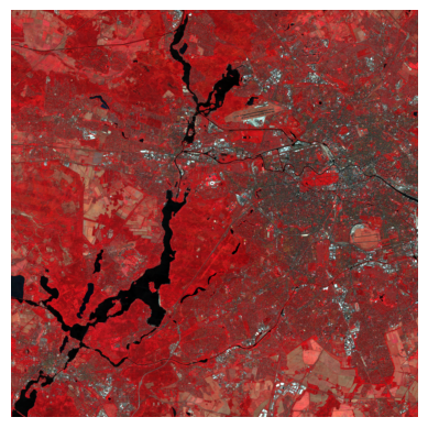
It is a good idea to visualize the Landsat image to see if we imported everything correctly. Let’s visualize the median image with the band combination NIR_Q50, RED_Q50, and GRN_Q50. To do that, we need to find the positions of those bands in the raster image. Again, we can write a list comprehension to loop over the band names, but that gives us only a single position. To understand what enumerate does click here does.
[i for i, x in enumerate(bnames) if x == "NIR_Q50"]
[14]
To get the positions of all three bands, we can write a nested list comprehension that combines looping over the band names of the raster and the band names of our desired band combination.
band_combination = ["NIR_Q50", "RED_Q50", "GRN_Q50"]
[[i for i, x in enumerate(bnames) if x == k] for k in band_combination]
[[14], [20], [8]]
This is to show you the power of list comprehensions in Python. Don’t be afraid to use them unless you have large datasets. We can also take advantage of the search functionality of pandas Series and DataFrames.
bc = pd.Series(bnames)
bc[bc.isin(["GRN_Q50", "RED_Q50", "NIR_Q50"])]
8     GRN_Q50
14    NIR_Q50
20    RED_Q50
dtype: object
geopy.plot_boa(lnd_img, bands=[14, 20, 8])
Data format#
In scikit-learn examples, it is customary to explicitly create the variables y (for the target vector or response) and X (for the feature matrix or predictors). You do not have to follow that convention, but it makes your code easier to read. Scikit-learn accepts numpy arrays and pandas Data.frames and Series. Here, we extract the target vector and feature matrix from the pandas Data.frame.
y = lucas['class']
y.shape
(332,)
X = lucas.drop(['class'], axis=1) # or X = lucas.iloc[:, 1:]
X.shape
(332, 36)
Feature scaling#
Feature scaling standardizes the predictors in your feature matrix. Feature scaling is important when predictors are highly varying in magnitude, e.g., when different units are involved. If such data is not scaled, machine learning algorithms that work with variances and/or distances will underperform because they will only utilize the features with the highest variance. To mitigate the problem, we rescale all features to the properties of a standard normal distribution with mean zero (μ = 0) and standard deviation one (σ = 1) using scikit-learn. The StandardScale() works in two steps: 1) the fit() estimates the distribution parameters mean and standard deviation, and 2) transform() applies the normalization. If you are not interested in keeping the distribution parameters, you can do the transformation in one step using fit_transform().
fittedScaler = StandardScaler().fit(X.astype('float32'))
X_scaled = fittedScaler.transform(X.astype('float32'))
X_scaled.shape
(332, 36)
Splitting data#
Now, lets split the data set int 50% training and %50 test set.
X_train, X_test, y_train, y_test = train_test_split(X_scaled, y, test_size=0.5)
Instantiate classifier#
First, we create an instance of the classifier. You can check the default hyperparameters with model.get_params().
svc_model = SVC()
svc_model.get_params()
{'C': 1.0,
 'break_ties': False,
 'cache_size': 200,
 'class_weight': None,
 'coef0': 0.0,
 'decision_function_shape': 'ovr',
 'degree': 3,
 'gamma': 'scale',
 'kernel': 'rbf',
 'max_iter': -1,
 'probability': False,
 'random_state': None,
 'shrinking': True,
 'tol': 0.001,
 'verbose': False}
Tuning#
Tuning is the process of maximizing an algorithm’s performance without overfitting or underfitting. Tuning is accomplished by selecting optimal hyperparameters from a model. A hyperparameter is a configuration external to the model and whose value cannot be estimated from data. Scikit-Learn offers two functions for optimizing hyperparameter tuning: GridSearchCV and RandomizedSearchCV. GridSearchCV performs an exhaustive search over specified parameter values for an estimator (or machine learning algorithm) and returns the best performing hyperparametric combination. RandomizedSearchCV uses randomized selections of hyperparameters and therefore tends to be less computationally expensive. SVM has two hyperparameters: C and gamma. Below, we conduct a grid search using three-fold cross-validation to evaluate the performance of each hyperparameter combination.
param_grid = {'C': [1, 5, 10, 40, 50, 60],
              'gamma': [0.0005, 0.001, 0.005, 0.006, 0.007]}
grid = GridSearchCV(svc_model, param_grid, cv=3)

grid.fit(X_train, y_train)
grid.best_params_
{'C': 5, 'gamma': 0.006}
From the fitted grid search object, we extract the best parameters (see above) and the best model (see below).
lc_model = grid.best_estimator_
lc_model.get_params()
{'C': 5,
 'break_ties': False,
 'cache_size': 200,
 'class_weight': None,
 'coef0': 0.0,
 'decision_function_shape': 'ovr',
 'degree': 3,
 'gamma': 0.006,
 'kernel': 'rbf',
 'max_iter': -1,
 'probability': False,
 'random_state': None,
 'shrinking': True,
 'tol': 0.001,
 'verbose': False}
Model Accuracy#
Model accuracy can be describe class-wise and overall. Precision (User’s accuracy) and Recall (Producer’s accuracy) describe the accuracy at the class level. Precision (User’s accuracy) describes the proportion of positive identifications that was actually correct:
\(Precision = \frac{TP}{TP+FP}\)
Recall describes the proportion of actual positives that was identified correctly:
\(Recall = \frac{TP}{TP+FN}\)
where, TP: true positives, FP: false positives, and FN: false negatives. To fully evaluate the effectiveness of a model, you must examine both precision and recall.
Apply model to the test data:
y_pred = lc_model.predict(X_test)
y_pred
array([5, 6, 6, 5, 4, 3, 5, 6, 6, 6, 6, 5, 3, 2, 5, 6, 5, 5, 6, 2, 3, 3,
       5, 5, 3, 4, 3, 5, 3, 2, 3, 2, 3, 3, 5, 5, 1, 5, 2, 6, 6, 4, 3, 5,
       6, 3, 1, 2, 5, 2, 5, 5, 3, 3, 2, 2, 4, 4, 5, 3, 1, 4, 5, 3, 1, 2,
       3, 3, 6, 6, 1, 2, 6, 2, 5, 6, 6, 3, 5, 6, 1, 5, 3, 3, 4, 2, 3, 5,
       5, 3, 2, 5, 3, 2, 5, 5, 5, 5, 5, 6, 3, 6, 3, 1, 6, 6, 6, 5, 1, 5,
       5, 5, 5, 6, 2, 3, 3, 6, 5, 3, 5, 3, 5, 1, 2, 5, 6, 6, 3, 5, 5, 1,
       6, 6, 5, 4, 1, 2, 3, 3, 3, 2, 6, 3, 4, 1, 4, 5, 6, 3, 6, 5, 6, 5,
       5, 3, 1, 5, 3, 3, 5, 1, 4, 4, 6, 6])
What is the probabiliy that a pixel is correctly classified?
print('Accuracy: %.4f' % metrics.accuracy_score(y_test, y_pred))
Accuracy: 0.8554
Confusion matrix#
metrics.confusion_matrix(y_test, y_pred)
array([[11,  0,  4,  1,  3,  0],
       [ 0, 18,  4,  0,  0,  0],
       [ 0,  1, 28,  0,  1,  0],
       [ 3,  0,  3, 11,  4,  0],
       [ 0,  0,  0,  0, 40,  0],
       [ 0,  0,  0,  0,  0, 34]])
Accuracy statistics#
aa_scores = metrics.precision_recall_fscore_support(y_test, y_pred)
aa_scores
(array([0.78571429, 0.94736842, 0.71794872, 0.91666667, 0.83333333,
        1.        ]),
 array([0.57894737, 0.81818182, 0.93333333, 0.52380952, 1.        ,
        1.        ]),
 array([0.66666667, 0.87804878, 0.8115942 , 0.66666667, 0.90909091,
        1.        ]),
 array([19, 22, 30, 21, 40, 34]))
Text report#
print(metrics.classification_report(y_test, y_pred))
              precision    recall  f1-score   support

           1       0.79      0.58      0.67        19
           2       0.95      0.82      0.88        22
           3       0.72      0.93      0.81        30
           4       0.92      0.52      0.67        21
           5       0.83      1.00      0.91        40
           6       1.00      1.00      1.00        34

    accuracy                           0.86       166
   macro avg       0.87      0.81      0.82       166
weighted avg       0.87      0.86      0.85       166
Map predictions#
Before we apply the model to the image, we need to transform the 3D-image with the shape (n_bands, n_row, n_col) into a 2D array of shape (n_row * n_col, n_bands). To achieve that, we first need to move the n_bands dimension to the last axis with transpose. Then we can collapse the first two dimensions with reshape. Finally, we need to transform the predictions back to 3-D.
# Get size of dimensions
n_bands, n_rows, n_cols = lnd_img.shape

# Transpose the array from (n_bands, n_rows, n_cols) to (n_rows, n_cols, n_bands)
flat_img = np.transpose(lnd_img, (1, 2, 0))

# Collapse the row and column dimension to get a 2-d array
flat_img = flat_img.reshape((n_rows * n_cols, n_bands))
print('Reshaped from {o} to {n}'.format(o=lnd_img.shape, n=flat_img.shape))
Reshaped from (36, 3000, 3000) to (9000000, 36)
Rescale image to mean 0 and unit variance.
fittedScaler = StandardScaler().fit(flat_img)
scaled_img = fittedScaler.transform(flat_img)
Make a prediction for each pixel using the flat image array:
lc_flat = lc_model.predict(scaled_img)
Reshape our classified flat array back into the image shape:
lc_map = lc_flat.reshape(lnd_img.shape[1:])
lc_map.shape
(3000, 3000)
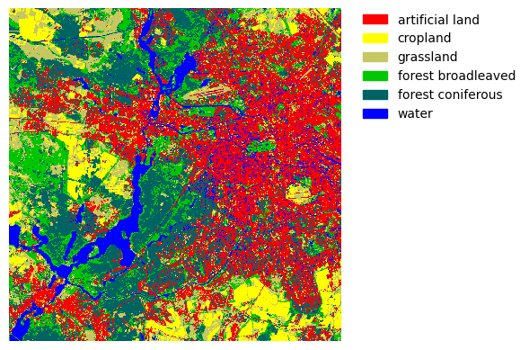
Map visualization#
The course module geopy has a small plot_map() function that also takes a list of labels and a dictionary of color codes as input. The color codes are of the format [red, green, blue, alpha], and the values range from 0 to 1.
lcColors = {1: [1.0, 0.0, 0.0, 1.0],  # Artificial
            2: [1.0, 1.0, 0.0, 1.0],  # Cropland
            3: [0.78, 0.78, 0.39, 1.0],  # Grassland
            4: [0.0, 0.78, 0.0, 1.0],  # Forest, broadleaf
            5: [0.0, 0.39, 0.39, 1.0],  # Forest, conifer
            6: [0.0, 0.0, 1.0, 1.0]}  # Water

labels = ['artificial land', 'cropland', 'grassland', 'forest broadleaved', 'forest coniferous', 'water']
geopy.plot_map(lc_map, lcColors, labels)
Map export#
We could just save the map as a standard 8-bit (np.ubyte()) image. The function below also embeds a predefined color ramp into the tif file. The color values range from 0 to 255.
colors = dict((
    (1, (255, 0, 0)),  # Artificial
    (2, (255, 255, 0)),  # Cropland
    (3, (200, 200, 100)),  # Grassland
    (4, (0, 200, 0)),  # Forest broadleaf
    (5, (0, 100, 100)),  # Forest conifer
    (6, (0, 0, 255))  # Water
))

out_file = os.path.join(outpath, "landsat_landcover_2015.tif")
geopy.writeArray(lc_map.astype(np.ubyte()), out_file, lnd_file, colors=colors)