Raster data#
In this part we finally get to work with some geographic data. Several weeks of the course are devoted to working with and manipulating raster data, which represent the most common type of data in our research. Looking at raster data and the different types of raster data we use, three examples come to mind:
Satellite imagery (continuous data)
Topographic information, e.g., a digital elevation model (continuous data)
Land cover (change) maps (categorical data)
We are very familiar with these types of data, and have visualized them in a GIS numerous times during our study career . However - for the purpose of completeness - we want to mention that there are another type of images that have some kind of geo-information, but that cannot be visualized in a GIS: so-called “geo-tagged” photos, that have one geo-coordinate associated with the entire picture. You will learn in this chapter, that also in case of the “common” raster files we don’t need much more than (a) one coordinate, and (b) information about the pixel size and the size of the entire image to visualize (and manipulate) these data.
We will do this using the Geospatial Data Abstraction Library (short: gdal). gdal is a computer software library for reading and writing raster and vector geospatial data formats, and is released under the permissive X/MIT style free software license by the Open Source Geospatial Foundation [GDAL/OGR contributors, 2023]. gdal can handle over 100 different raster-formats (through so-called drivers), and in addition offers a number of of built-in functions (e.g., gdal_translate, gdal_proximity).
Important
Important to recognize is that gdal really only helps us in accessing geospatial information and bring it into a form that allows us to manipulate the data. Specifically, and for our context, using gdal we will access raster-files and load their content into numpy-arrays. To do that, however, we need to first learn something about the raster format.
Gdal raster model#
We will use now some time to get to know how raster. In gdal the general structure of a raster file is as follows:
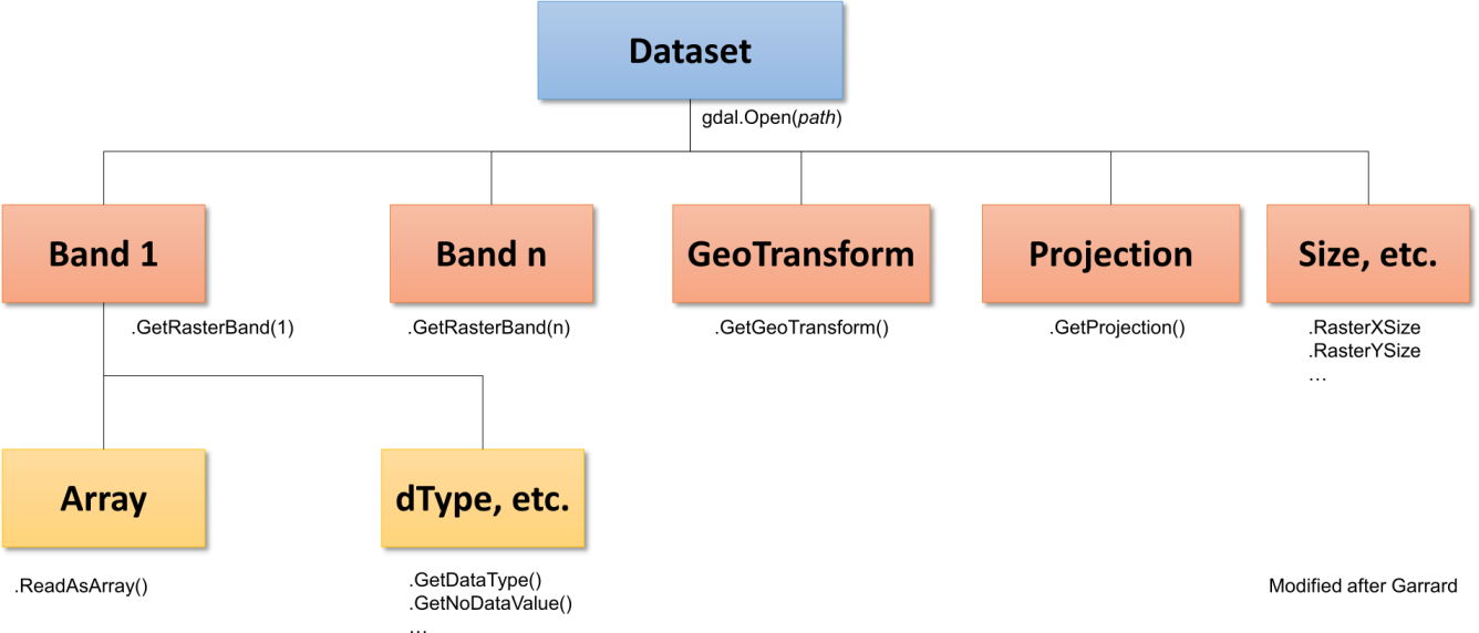
Fig. 1 Overview about the gdal raster structure. For more info and background visit the gdal documentation and see Garrard (2016) Geoprocessing in python chapter 9 (available in moodle).#
You can imagine the structure in different levels. On the first level (blue) the dataset is being accessed, using gdal.Open(path). Important is that you create a variable, which points to the dataset. In addition, you will have to import the gdal library. A potential code look like that:
from osgeo import gdal
gdal.UseExceptions()

path = "D:/OneDrive - Conservation Biogeography Lab/_TEACHING/__Classes-Modules_HUB/M8_Geoprocessing-with-python/02_RasterData/WS_23-24/Assignment02/"
ds = gdal.Open(path + "tileID_410_y2000.tif")
ds
<osgeo.gdal.Dataset; proxy of <Swig Object of type 'GDALDatasetShadow *' at 0x000002457F4E2A90> >
Looking at the output, you see that the variable ds is just a pointer to the actual file, and nothing has been moved to the memory. Now, let’s access some more information. We start with the size of the rasterfile. The general syntax here is that you call the raster object ds followed by . and the method.
cols = ds.RasterXSize
rows = ds.RasterYSize
nbands = ds.RasterCount
cols, rows, nbands
(1529, 1380, 1)
The raster has 1529 columns, 1380 rows and 1 band. So, nothing really spectacular and nothing we haven’t been looking at. What is important to recognize here is that the three variables are now actually stored and do not represent a pointer. Now, we check in which projection the raster is stored - we do this using the method .GetProjection()
pr = ds.GetProjection()
pr
'GEOGCS["WGS 84",DATUM["WGS_1984",SPHEROID["WGS 84",6378137,298.257223563,AUTHORITY["EPSG","7030"]],AUTHORITY["EPSG","6326"]],PRIMEM["Greenwich",0,AUTHORITY["EPSG","8901"]],UNIT["degree",0.0174532925199433,AUTHORITY["EPSG","9122"]],AXIS["Latitude",NORTH],AXIS["Longitude",EAST],AUTHORITY["EPSG","4326"]]'
The output here comes as a Wellknown Text (Wkt). For the moment this is nothing to be too concerned of, but generally remember that when you create a new rasterfile and you want to assign a projection, that projection needs to be in form of a Wellknown Text. There are tools to convert e.g., epsg codes into wkt, but we cover this later during the course or during the final class project.
Geotransform#
Next, we look at the affine transformation. This is for this week the most important piece of information (besides the number of columns and rows), and we will spend now some time to look at it. I store the information as the variable gt to build a mental connection to the method we are calling to get this information .GetGeoTransform()
gt = ds.GetGeoTransform()
gt
(-63.86859973338657,
 0.00026949458523585647,
 0.0,
 -24.446662310500248,
 0.0,
 -0.00026949458523585647)
The ouput is a tupel containing a total of 6 pieces of information:
the x-coordinate of the upper left corner of the raster file. This coordinate has to correspond to the coordinate system that the entire raster is stored
The pixel size is x-direction. The units have to correspond to the coordinate system as well.
The rotation of the pixel in x-direction \(\rightarrow\) I have never encountered a case where this value is not 0
The y-coordinate of the upper left corner
Rotation of the pixel in y-direction \(\rightarrow\) see point 3.
The pixel size in y-direction.
You notice probably two important aspects: (1) the upper left coordinate seems to be important, (2) the pixel size is once noted as a positive number, and once as a positive number. Both points are related to each other, and the figure visualizes this - can you explain now why 2. and 6. have the same absolute value but different signs?
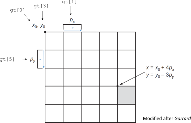
Fig. 2 Overview about the elements of the function call .GetGeoTransform().#
As a preview and an encouragement for thinking to our course and exercise, we want you to think about a couple of more questions.
How can one calculate the geo-coordinate of the other four corners of a raster file?
Could you apply the same strategy to get the geo-coordinate of the center?
How can considering the affine transformation help you working with two raster files of different extent?
Load raster into an array#
Now, all that is left is to find out how to load the data into memory to be able to work on this. Generally, we use the pacakge numpy to manipulate the data, so what we need to do is find a method that gets the data and loads it into a numpy array. The way we do this is by accessing the last method in the orange level .GetRasterBand(), followed by the method .ReadAsArray(). You can call them separately, like in the examples below, or you can combine them within one call .GetRasterBand().ReadAsArray()
The argument for the function .GetRasterBand() is simple: all you need to provide is an integer value for the band you want to access \(\rightarrow\) caution: here, we don’t have zero-based counting. The first band has the index 1. The return value is again only a pointer to the respective band (similar to the function gdal.Open()). We have not yet loaded any data into memory.
rb = ds.GetRasterBand(1)
rb
<osgeo.gdal.Band; proxy of <Swig Object of type 'GDALRasterBandShadow *' at 0x00000245B1DAC1B0> >
If you follow again the flowchart from above, we can also now check for the data type of the raster. If you go back to the Python basics chapter, you remember that there are different data types depending on the precision and the type of values. In gdal, these are coded with numeric values. Below you find a list for the most common data types. Can you think of typical data that are stored with these data types?
Code |
Data Type |
Range of possible pixel values |
|---|---|---|
1 |
GDT_Byte |
0 - 255 |
2 |
GDT_UInt16 |
0 - 65535 |
3 |
GDT_Int16 |
-32768 - 32767 |
4 |
GDT_UInt32 |
0 - 4294967295 |
5 |
GDT_Int32 |
-2147483648 - 2147483647 |
6 |
GDT_Float32 |
Decimal values with single precision -3.4 × 1038 to 3.4 × 1038 (7-8 decimal digits) |
7 |
GDT_Float64 |
Stores decimal values with double precision for higher accuracy -1.7 × 10308 to 1.7 × 10308 (15-17 decimal digits) |
dtype = rb.DataType
dtype
5
The argument for loading the band into an array are slightly more complex. You need to provide four values (in that order):
origin_x: the x-coordinate of the upper left corner of the part you want to load from the array. In the example below we want to load the entire array, so the origin has the coordinate (0,0), and the value fororigin_xhence is 0.origin_y: same as fororigin_xsliceSize_x: the number of columns you want to load from the array \(\rightarrow\) important: this refers to array-coordinates (using zero-based counting) and not to geo-coordinates. The value is an integer value and is often confused with the lower right coordinate; likely because when you load an entire array, then the lower right array-coordinate is the same as the value forcols.sliceSize_y: same as forsliceSize_x, but here for the y-direction. Important: because we are talking about slice sizes and not coordinates, this value can never be negative!
In the example below, we load the entire rasterband into an array:
ds_arr = rb.ReadAsArray(0, 0, cols, rows)
ds_arr
array([[10752, 11593, 12625, ...,  4840,  4553,  4645],
       [10811, 12021, 12399, ...,  5314,  5285,  5115],
       [12378, 12295, 12916, ...,  5541,  5561,  5925],
       ...,
       [ 4308,  3952,  3796, ...,  7751, 10913, 12762],
       [ 4133,  3667,  3877, ...,  7924,  9907, 12482],
       [ 5173,  5012,  4916, ...,  8940, 11699, 13095]], dtype=int32)
Now, we have loaded the raster data into numpy and are ready to work with the data. We will only apply some smple functions this week to calculate simple statistics, such as the mean value of the entire array. During the next weeks we will become gradually more and more complex with our operations. However, the steps to be taken so that actual data can be manipulated, are always the same once described here.
Creating a raster file#
Now, that we know (a) what the different elements of a raster file are, and (b) how to load a raster into an array; we want to understand how to create a raster. Generally, to create a raster, we need the following pieces of information:
The size of raster (i.e., rows, columns, number of bands)
A coordinate reference system
The affine transformation
In addition, we need to define in which data format we want to store the data. The two formats I personally use most are GTiff and MEM. The first one is one you probably already know: GeoTiff, which is a Georeferenced Tagged Image Format File. Probably in several instances you already had contact with this type of file. The other one, is a memory format. Here, the raster file is not written to disc, but only into the RAM. This can come in handy, e.g., when you only want to create a temporary raster, or when you have several operations on the same raster file; because operations that happen within the memory are always faster (in terms of reading and writing) compared to the hard disc. In gdal, the formats are organized in form of drivers, which need to be defined beforehand:
drvR = gdal.GetDriverByName('GTiff')
drvMemR = gdal.GetDriverByName('MEM')
Below you find an example for each. You will notice that except for the first line (i.e., where I create the file) everything is the same. I show it anyways to get you again exposed to the standardized language and formats that gdal is using. In both cases I will create a new raster file that is identical to the one we have opened before. While it is thematically meaningless, I find it easier to follow:
# Creation in Memory
memRas = drvMemR.Create('', cols, rows, nbands, dtype)
memRas.SetProjection(pr)
memRas.SetGeoTransform(gt)
0
# Creation on drive
driveRas = drvR.Create(path + "TestFile.tif", cols, rows, nbands, dtype)
driveRas.SetProjection(pr)
driveRas.SetGeoTransform(gt)
0
That’s all. It looks pretty simple - and it truly is! Although we are taking here a maybe not so useful example, the technique for creating files is always the same. Therefore, we encourage you to familiarize yourself with these techniques.
As a last bit, we want to introduce you to a technique with which we can copy a raster dataset from the drive into memory. We often do this, when we will do multiple operations with a rasterfile and do not want to sequentially read in individual bands. Instead, we want to copy the full raster into memory. This of course it depends on the computer you have available (most importantly the available RAM). But assuming you have RAM available and you want to do several sequential operations this will greatly speed up your overall process. Generally you can think of the rule: one long access to the physical disc goes faster than multiple short accesses.
I already wrote the code in form of a function; you have learned already how one can build a function in the Python basics chapter, and this is an application to geodata.
def OpenRasterToMemory(path):
    '''
    Function that copies a local raster file into memory.
    PARAMETER
    -----------
    path : full file-path to the raster stored on the hard disc (string)

    RETURNS
    -------
    Raster object in Memory
    '''
    drvMemR = gdal.GetDriverByName('MEM')
    ds = gdal.Open(path)
    dsMem = drvMemR.CreateCopy('', ds)
    return dsMem
With this, you are pretty much set to do everything with raster files. Make sure, you memorize this and keep practicing! From reading alone noone has ever learned coding!
Last notes#
We focus here on the general raster structure and the methods in gdal to access the different elements of the structure. Of course you can also do a lof of more cool stuff, including (1) reproject images, (2) rasterize vector data, etc. Many of the functions we will touch upon in this course and in this online script, but others not. We encourage you to continue reading, using some additional sources, e.g.,
The book by Garrard. It is a bit outdated in some aspects but has still some nice information, particularly regarding the affine transformation
Lastly, you probably came across already some wrapper functions, such as the rasterio package. These are all really cool packages. Why we try to avoid these packages here to large extents is that we want you to understand the structure of a raster file and how to maneuver the different pieces of information to get to our result. Packages such as rasterio do many of the things under the hood. This is cool when number of files you work with is low and/or the files themselves are relatively small (in terms of their size). When it comes to large datasets, however, we need to be efficient in how to access data and often we only access parts of the data and can logically exclude other parts. Using wrapper functions makes this often more difficult (or impossible) which is why we want you to focus on the core elements of raster processing. You also don’t run into trouble if the packages are deprecated or not maintained, hence resulting in a lack of compatibility to other functions.