11. Time series analysis
Learning goals
- Investigate long and dense time series
- Understand the concepts of land surface phenology and change
- Interpret change trajectories
Background
Long and dense time series
Integrating the temporal dimension into remote sensing image analyses allows to answer relevant and exciting geographical questions. Several satellite-based optical sensors allow for tracking the Earth´s surface over several decades by means of long and dense times series. With long and dense we refer to time series representing multiple years (i.e. multi-annual) with satellite observations of high temporal density within each year (i.e., intra-annual).
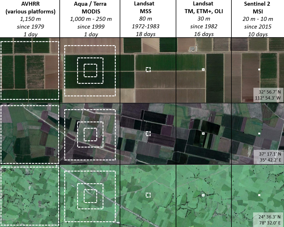
The figure below shows a selection of satellite missions and sensors and their characteristics regrading image acquisition of long and dense time series. AVHRR and MODIS provide near-daily global coverage at coarse spatial resolution, while Landsat and Sentinel-2 provide images of higher spatial resolution but with lower revisit frequencies. Differences between these sensors also arise in terms of the temporal coverage.
AVHRR for instance captures the globe sice 1979, while the first MODIS sensor was launched in 1999. The Landsat family of sensors is operational since 1982 (or 1972 but with the MSS sensor which has lower spatial resolution and less spectral bands). Data acquired from the European Sentinel sensors are available only for recent years, limiting their use in long time series analyses.
Land surface phenology
For analyzing long and dense time series, the multi-spectral signal is commonly reduced to a desired target indicator, such as a vegetation index. Analyzing, for instance, a time series of NDVI facilitates interpretation and analysis as compared to analyzing time series of multiple spectral bands.
MOD13Q1 is a analysis-ready product providing NDVI (and EVI) measurements at 16-day intervals and in 250m (or 500m) spatial resolution for any location on the globe. It also comes with a quality layer indicating if an observation represents good data (clear sky, not quality issues), marginal data (some quality issues, may be of limited use), or if a pixel is covered by snow, ice, or clouds. The below video shows a global NDVI time series derived from the MODIS product MOD13Q1 (Version 6).
We can also get a different perspective on such time series by looking at a single pixel. Below, you look at a dense time series of Landsat NDVI values for three consecutive years for a deciduous forest in the Wuhlheide. The dots represent the actual NDVI values, whereas the gray line represents an interpolation between these values.
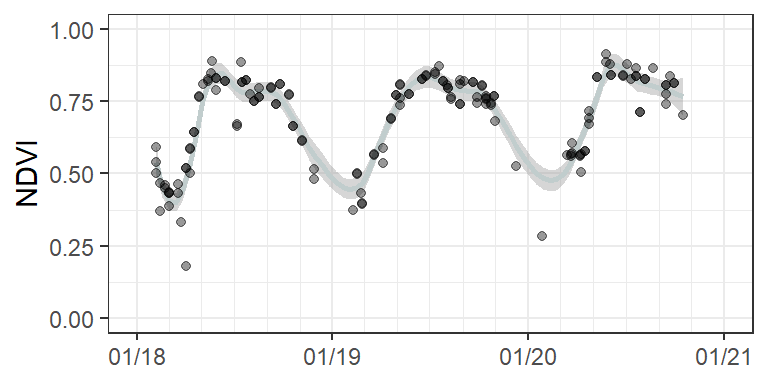
This graph reveals the seasonality of the forests, with increasing NDVI values in the green-up phase in spring, high NDVI values (>0.75) during the peak phenological phase in late spring until early autumn and decreasing NDVI values during the senescent phase in late autumn. Remember that we are looking at a 30x30m pixel, which may contain the signal from several tree canopies but also understory, such as shrubs or herbaceous vegetation in the openings of the canopy or under the trees when leaves are shed. Scientists in the remote sensing community refer to this mix of signal from various surface types as land surface phenology.
Land surface change
The seasonal component of long and dense time series was illustrated in the previous Wulheide example, representing the land surface phenology of a intact broadleaf forest stand. Many ecosystem are, however, subject to land surface change processes that are additionally captured by the time series. The ability to quantify these land surface changes largely depends on the lengths of the time-series back in time, and thus on the temporal coverage of the underlying satellite/sensor system. For example, pioneer deforestation patterns or land degradation processes can be traced back to the 70ties with the Landsat system, while latest disturbance induced changes like fires or logging can also be analyzed with Sentinel-2 data.
For analyzing land surface change processes, long and dense time series (but also only long time series with a single yearly observation) lead to characteristic trajectories, which are schematically represented in the figure below.
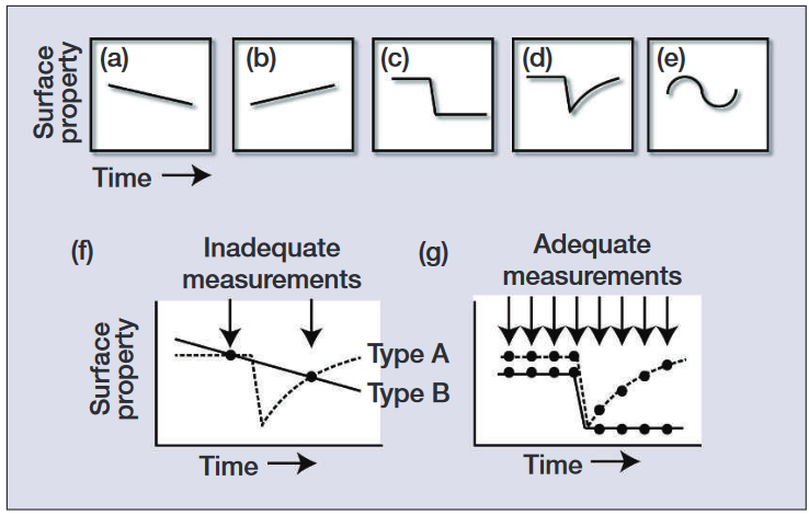
Kennedy et al. (2014); doi:10.1890/130066
For a given target indicator such as the NDVI, we see a gradual decrease (a), a gradual increase (b), an abrupt decrease from high to low (c), an abrupt decrease from high to low with subsequent gradual increase (d), and a cyclic pattern (d). In the given context, these trajectories can be related to specific change processes such as a loss of green cover due to land degradation (a), an increase in green cover due to vegetation encroachment (b), replacement of forest by urban land (c), logging of forest with secondary forest regrowth (d). The cyclic pattern (e) represents a special case as it resembles the seasonal component and therefore rather represents land surface phenology. However, there are also cyclic land surface change processes that stem from regular management practices, e.g. removal of woody-vegetation to reduce fire risk.
Interpreting long and dense time series
In summary, long and dense time series contain multiple components that need to be considered during their interpretation and analysis:
- land surface phenology: seasonality of vegetation on a land surface
- land surface change: gradual and abrupt changes of land surfaces
- measurement uncertainties related to
- cloud contamination,
- under- / overestimated atmospheric effects
- absolute or multi-temporal geometric misregistration
All these components merge into a single time series signal. We need a sufficient temporal resolution of remote sensing observations to mitigate cloud cover and to match the phenology and the change processes to be monitored. Long and dense time series provide an analytic basis for such monitoring. Often, the different components can be well identified visually. Today, we want to interpret NDVI time series from selected locations around the world.
Download and unzip the session
materials from our shared repository. We prepared five time-series
plots (fe1_s11_data/Exercise_S11_MODIS-NDVI.pdf) showing
the NDVI of selected sites across the globe between 2006 and 2022, for
instance:
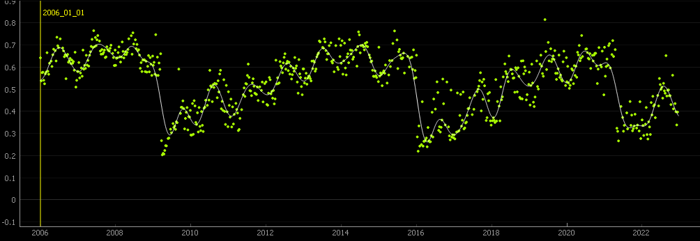
The NDVI time series is derived from the
MOD09Q1.061 Terra Surface Reflectance 8-Day Global 250m
product using the GEE
Time Series Exlorer plugin in QGIS/EnMAP-Box. Later in the
assignment you will work with the GEE Time Series Exlorer
yourself, but first take a look at the provided time series plots and
descriptions in the pdf-file.
-
Exercise
Try to match the correct pairs of land surface description (1-5) and corresponding NDVI time series plot (A-E)! Provide reasoning for your choice and describe the processes in terms of their characteristic time series trajectories.
Assignment
The goal of this assignment is to visualize and interpret individual pixel time series of MODIS-derived NDVI. You will make use of the GEE Time Series Exlorer plugin in order to extract the data and graphs of the 8-day NDVI time series from existing MODIS products for each location. The plugin is developed by members of our EOLab and enables interactively exploring temporal raster data available in the Google Earth Engine (GEE).
After successfully installing the GEE Time Series Exlorer
plugin, open the plugin in the EnMAP-Box by clicking  :
:
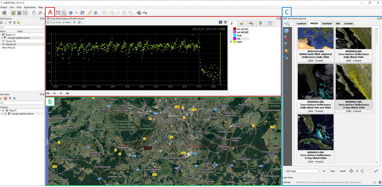
The plugin features three main windows: A Plot and
visualization settings window, B Map view and
C Data catalogue and settings window. Explore and find out
how to use the plugin with the help of the video below (link):
How to extract time series
As illustrated during the seminar and in the video above, the GEE Time Series Exlorer plugin comes with many predefined datasets (“Image Collections” in GEE terms). Today we want to access the MODIS Surface Reflectance 8-Day Global 250m product.
Select the MODIS product:

> MODIS > MOD09Q1.006 Terra Surface Reflectance 8-Day Global 250mAs mentioned above, pixels of optical data are often contaminated by clouds or cloud shadows. Preprocessed datasets such as the MODIS product come with quality information for each pixel, allowing to identify cloud/cloud shadow impacts and remove them for further analyses if needed. Accordingly, we want to filter our dataset to remove pixels containing clouds, cloud shadows and snow. Under

>
> Surface Reflectance 250m state flags [State]select:
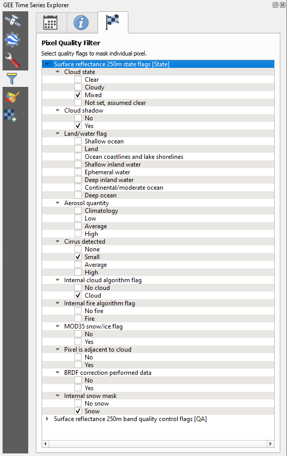
Select the
NDVIin the visualization window under theLegendsettings
Now navigate to a region of your choice in the map view window and retrieve the NDVI time series by left-clicking into the map (Make sure the identify cursor is activated
 ).
).
Interpretation of selected sites
- The following table consists of 8 different locations distributed
around the globe which are also compiled in the
.gpkgof today’s materials:
| point ID | Latitude | Longitude | Quality |
|---|---|---|---|
| 1 | -6.6197 | -55.1835 | Show good quality |
| 2 | 30.0908 | 31.1917 | Show good quality |
| 3 | 22.1954 | 76.6071 | Show all |
| 4 | 22.2731 | 28.6997 | Show all |
| 5 | 50.8883 | 6.5388 | Show good quality |
| 6 | -31.1007 | 152.4433 | Show good quality |
| 7 | 13.1491 | 80.1645 | Show all |
| 8 | 36.7129 | -2.7875 | Show all |
Open the
coordinates.gpkgin the map viewPlease use the following table template to interpret the time series of each location.
| Point ID | Location | Land cover | Land surface phenology | Land surface change | Data availability |
|---|---|---|---|---|---|
| 1 | … | … | … | … | … |
| 2 | … | … | … | … | … |
| 3 | … | … | … | … | … |
| … | … | … | … | … | … |
With regard to your visual assessment of each point location in Google Earth, answer the following questions:
- Which region are you looking at (e.g., continents, biomes, countries, etc.)?
- Which land cover type(s) are we looking at (keep in mind the 250m spatial resolution of the MODIS product)?
Now focus on the results of your GEE Timeseries Exlorer request. You can visit the different sites, decide if you want to only visualize good quality observations (no clouds, snow, ice, water, radiometric saturation or other uncertainties). For some points, you will need to restrict to good quality observations, for others it does not make sense.
Interpret the time series from a geographical perspective and answer the following questions:
- What are the general patterns of the vegetation seasonality (e.g., timing, amplitude)?
- Can you identify long-term trends or abrupt changes?
- How do you judge the data availability (e.g., overall availability, seasonal data density)
Note that you may use additional sources (Google Earth historic images, Wikipedia, literature) to better understand and describe the processes you are looking at
Submission
- Please upload your interpretation (table) and screenshots (right-click in plot window allows for export, too) of the time-series graphs as a pdf to moodle.
Copyright © 2023 Humboldt-Universität zu Berlin. Department of Geography.
![]()