- Learning goals
- Raster data in R: the
terrapackage - Reading raster data
- Plotting raster data
- Raster stacking
- Raster writing
- Raster indexing
- Data types
- Raster algebra
- Reprojecting and spatial subsetting
- Assignment
- Submission
3. Image properties II
Learning goals
In the last session you were introduced to raster data, heard about
some basic properties and data formats, and learned how objects appear
in true- and false-colour representations. Today we will deepen our
understanding of raster data and learn how to handle it in R. We will
learn about the terra package, which is a powerful tool for
handling raster data in R. Specifically, we will look into:
- Reading raster data into R and revisiting metadata
- Visualizing rasters in R
- Raster stacking: Combining single-band to multi-band rasters
- Writing raster data to disc (…and why data types are important)
- Basic raster algebra: Manipulating raster values
- Reprojecting and resampling: Changing extent, coordinate system and resolution
 Why code?
Why work with geospatial data, or any data really, in a programming environment and not only stick with Graphical User Interfaces (GUIs) like QGIS? For us it is particularily the flexibility of processing data and not being restricted to predetermined tools and functions. Also we often find ourselves having to apply a certain chain of processes repeatedly over different data. It is particularily the reusability of code that outcompetes working in a GUI in terms of efficiency. Last, getting acquainted with any programming language is generally a great and much in demand skill.
Help with coding
Once you enter the world of programming and you will come across syntax errors or tasks in which you need help with writing code. You are learning new a language after all. Good news is there are many excellent tutorials and community feedback out there which will help you tremendously in achieving your tasks. One great resource is the Stack Overflow community where people can ask code related questions and seek help from fellow (advanced) programmers. Make sure to Google your problem and chances are very high you come across a forum entry precisely matching your needs. Then, of course, there is ChatGPT. Last, do not unterestimate your own problem solving skills which will grow quickly in terms of coding with time spent doing so.
Raster data in R: the terra package
Last week you learned that raster data stored in image formats are
essentially a collection of pixels stored along rows and columns in
matrices or tables. But how do we deal with such data in R? The
terra package offers useful classes and functions which
facilitate raster data handling in R. It allows us to access file
characteristics before loading data into memory, manipulate coordinate
reference systems and spatial extents. We can use it to perform raster
algebra, to combine raster and vector datasets (e.g. ESRI shapefiles),
or to convert raster files into matrices, which then become compatible
with base-R functions to manipulate data, do statistics, develop models,
and much more. The terra package supersedes the older
raster package developed by the same team of authors.
Because raster has been around for a longer time,
dependencies with some packages may still exist. But development of
raster will eventually be stopped at some point.
Installation
With your R console opened in RStudio you can install and then load the terra package like any other package in R as follows:
# install the terra package
install.packages('terra')

# load the package to get access to the package's routines/functions in your environment
library(terra)
terra classes and functions
terra introduces new classes (or structures) to your R
environment, the most important of them being:
SpatRasterto handle raster dataSpatVectorto handle spatial vector data, i.e., points, lines, polygons.SpatExtentto handle information on spatial extents
The full suite of functions found in the terra package
can be accessed by typing help(package = "terra") into the
console or by browsing the package
documentation or package’s
webpage.
Reading raster data
Once the terra package is loaded, we can start reading
geospatial data into R. Let’s start with last week’s Landsat-8 image
covering Berlin
(LC08_L1TP_193023_20190726_20200827_02_T1_int16.tif).
To create a SpatRaster object in R, we need to the
filepath to the image and then use terra’s rast()-function
to read it into our environment.
# create a new string variable containing the path to your image file
path_landsat <- "data/Landsat-8/LC08_L1TP_193023_20190726_20200827_02_T1_int16.tif"
# read the file into raster object
img_landsat <- rast(path_landsat)
# print metadata to console
print(img_landsat)
## class : SpatRaster
## dimensions : 1840, 2171, 6 (nrow, ncol, nlyr)
## resolution : 30.00639, 30.00728 (x, y)
## extent : 360793.1, 425937, 5794470, 5849683 (xmin, xmax, ymin, ymax)
## coord. ref. : WGS 84 / UTM zone 33N (EPSG:32633)
## source : LC08_L1TP_193023_20190726_20200827_02_T1_int16.tif
## names : BLU, GRN, RED, NIR, SW1, SW2
## min values : 639, 371, 227, 60, 23, 16
## max values : 5603, 5984, 6728, 7454, 11152, 8946 Absolute
vs. Relative Paths
When working with file paths in R and
RMarkdown, it’s important to understand the difference between absolute
and relative paths.
Absolute Paths: These paths specify a location from
the root directory. They are complete and unambiguous, but they can make
your code less portable. For example,
C:/Users/You/Documents/data/Landsat-8/LC08_L1TP_193023_20190726_20200827_02_T1_int16.tif
is an absolute path.
Relative Paths: These paths specify a location
relative to the current working directory. They are more portable and
flexible, especially when sharing code with others. For example,
data/Landsat-8/LC08_L1TP_193023_20190726_20200827_02_T1_int16.tif
is a relative path.
# print metadata to console
print(img_landsat)
## class : SpatRaster
## dimensions : 1840, 2171, 6 (nrow, ncol, nlyr)
## resolution : 30.00639, 30.00728 (x, y)
## extent : 360793.1, 425937, 5794470, 5849683 (xmin, xmax, ymin, ymax)
## coord. ref. : WGS 84 / UTM zone 33N (EPSG:32633)
## source : LC08_L1TP_193023_20190726_20200827_02_T1_int16.tif
## names : BLU, GRN, RED, NIR, SW1, SW2
## min values : 639, 371, 227, 60, 23, 16
## max values : 5603, 5984, 6728, 7454, 11152, 8946You can see that the print(img_landsat) command prints a
couple of image properties or metadata to the console you are
already familiar with.
Metadata Metadata is data about data. It includes the already familiar image properties as well as conditions recorded during data acquisition (e.g. sun angle, time of day), or information added during pre-processing to reconstructr how the data came to be. Metadata are either stored as part of an integrated data format, i.e. stored in the same file, or as an additional file accompanying the image data. Example GeoTIFF: metadata stored within .tif image. Displaying metadata possible with specific metadata reader (e.g. QGIS Layer properties, R functions).
Plotting raster data
Next, we can visualize our image by simply using the
plot() function:
plot(img_landsat)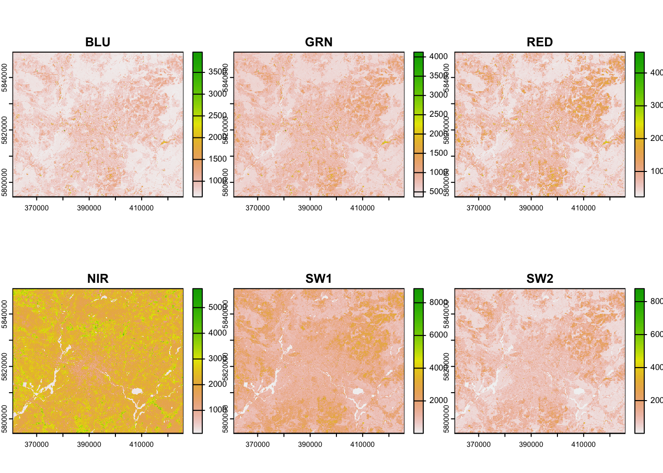
By default, this creates a single plot for each band without contrast
enhancement and using a single-band pseudocolour
representation. If we would like to create a multi-band RGB composite,
we can use plotRGB() to achieve this.
Exercise 1
help(plotRGB) or ?plotRGB into the console to
learn how to use this function, i.e. which arguments of the
function you need. As a hint, you need five arguments of the function.
Below you find the desired visual result.
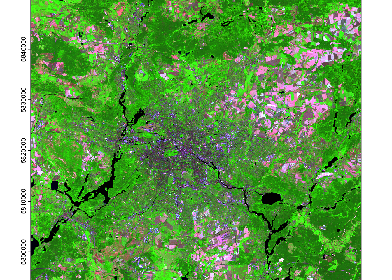
Inspecting ?plotRGB reveals we need the arguments
x (= the spatial raster object), r,
g, b (the position or index of the bands), and
stretch (the contrast stretching method).
plotRGB(img_landsat, r=6, g=4, b=3, stretch = "lin", axes=TRUE) # we can also set axes=TRUE to display the coordinatesRaster stacking
The Landsat-8 image we have used so far is provided as a single multi-band image, but this is not always the case. Optical remote sensing data for a specific region and time is initially stored and provided in multiple single-band images, each file corresponding to a single spectral band recorded by the sensor. To illustrate this, we will now take a look at Sentinel-2 data acquired over Berlin on the same day as the Landsat-8 image. Sentinel-2 is also a multispectral sensor, but features different spatial, spectral, and temporal resolution compared to Landsat-8. Sentinel-2 offers up to 10 meter spatial resolution (compared to the 30 meter Landsat data), allowing for capturing finer spatial grain, which can be advantageous in a heterogenous mosaic landscape like an urban environment.
The Sentinel-2 data is already available in your data folder of last’s and today’s session. You can inspect the single-band GeoTIFF-files in your file explorer, the content of which looks like this:
## [1] "data/Sentinel-2/SEN2A_BOA_20190726_BLU_flt32.tif"
## [2] "data/Sentinel-2/SEN2A_BOA_20190726_GRN_flt32.tif"
## [3] "data/Sentinel-2/SEN2A_BOA_20190726_NIR_flt32.tif"
## [4] "data/Sentinel-2/SEN2A_BOA_20190726_RED_flt32.tif"
## [5] "data/Sentinel-2/SEN2A_BOA_20190726_SW1_flt32.tif"
## [6] "data/Sentinel-2/SEN2A_BOA_20190726_SW2_flt32.tif"
Exercise 2
Before we deal with raster stacking, let us
first screen a single Sentinel-2 image file in QGIS to get a visual
impression of the data.
- Open QGIS
- Add the Landsat-8 image to QGIS and visualize the near-infrared (NIR) band as contrast enhanced greyscale image.
- Add the Sentinel-2 NIR band to QGIS (a window will likely appear, asking which coordinate transformation to apply. Leave at default and click OK) and visualize it as contrast enhanced greyscale image.
- Compare the two images in terms of spatial resolution: Drawing from the lecture series, which “problem” is less pronounced in the Sentinel-2 data compared to Landsat-8 data?
Back to stacking. The Sentinel-2 data is currently stored in single band images for each band. Our goal is now to create a multiband image - like the Landsat image - that contains all the bands in a single file. This process of merging bands into a multiband image is frequently called raster stacking.
Raster
stacking Raster stacking is the process of combining multiple single-band image files into a single multi-band image file. Images must share the same spatial extent and pixel resolution when stacked.
Let us take a look how to create a raster stack in R. We will illustrate two of many approaches, all leading to the same result, but as always there are multiple ways to achieve the same goal when programming:
Option 1: We create a SpatRaster object
for each single using rast() and combine the results into a
multi-band image using c():
img_BLU <- rast('data/Sentinel-2/SEN2A_BOA_20190726_BLU_flt32.tif')
img_GRN <- rast('data/Sentinel-2/SEN2A_BOA_20190726_GRN_flt32.tif')
img_RED <- rast('data/Sentinel-2/SEN2A_BOA_20190726_RED_flt32.tif')
img_NIR <- rast('data/Sentinel-2/SEN2A_BOA_20190726_NIR_flt32.tif')
img_SW1 <- rast('data/Sentinel-2/SEN2A_BOA_20190726_SW1_flt32.tif')
img_SW2 <- rast('data/Sentinel-2/SEN2A_BOA_20190726_SW2_flt32.tif')

img_s2 <- c(img_BLU, img_GRN, img_RED, img_NIR, img_SW1, img_SW2)
Option 2: We provide the filepaths to the
rast() function directly as a vector (note that we
explicitly consider the order, i.e. we start with blue and end with
shortwave-infrared 2):
# Create a vector using c() containing the filepaths;
l_bands <- c(
  'data/Sentinel-2/SEN2A_BOA_20190726_BLU_flt32.tif', 'data/Sentinel-2/SEN2A_BOA_20190726_GRN_flt32.tif',
  'data/Sentinel-2/SEN2A_BOA_20190726_RED_flt32.tif', 'data/Sentinel-2/SEN2A_BOA_20190726_NIR_flt32.tif',
  'data/Sentinel-2/SEN2A_BOA_20190726_SW1_flt32.tif', 'data/Sentinel-2/SEN2A_BOA_20190726_SW2_flt32.tif'
)
# provide vector of filenames to rast() function; check "?rast" for details
img_s2 <- rast(l_bands)
print(img_s2)
## class : SpatRaster
## dimensions : 4977, 6279, 6 (nrow, ncol, nlyr)
## resolution : 10, 10 (x, y)
## extent : 4524946, 4587736, 3248660, 3298430 (xmin, xmax, ymin, ymax)
## coord. ref. : ETRS89-extended / LAEA Europe (EPSG:3035)
## sources : SEN2A_BOA_20190726_BLU_flt32.tif
## SEN2A_BOA_20190726_GRN_flt32.tif
## SEN2A_BOA_20190726_RED_flt32.tif
## ... and 3 more source(s)
## names : SEN2A~flt32, SEN2A~flt32, SEN2A~flt32, SEN2A~flt32, SEN2A~flt32, SEN2A~flt32
## min values : ? , ? , ? , 0.0065, 0.0056, ?
## max values : ? , ? , ? , 0.9975, 0.9874, ?Raster writing
Now that we have created a raster stack we would like to save the
SpatRast object to disc as a GeoTIFF file. We can do this
using the writeRaster function.
Exercise 3
Take a look at the writeRaster help page. There are two
mandatory arguments which the function expects, the remainder are
optional and come with default settings. Try writing your raster stack
into your Sentinel-2 folder while choosing a meaningful filename.
# learn how to use the function
?writeRaster
# provide the necessary arguments to save your image to disc
writeRaster() button at
the top panel and clicking somewhere into the map view. If you
right-click, select “Identify All” to inspect the values of both images.
button at
the top panel and clicking somewhere into the map view. If you
right-click, select “Identify All” to inspect the values of both images.
Raster indexing
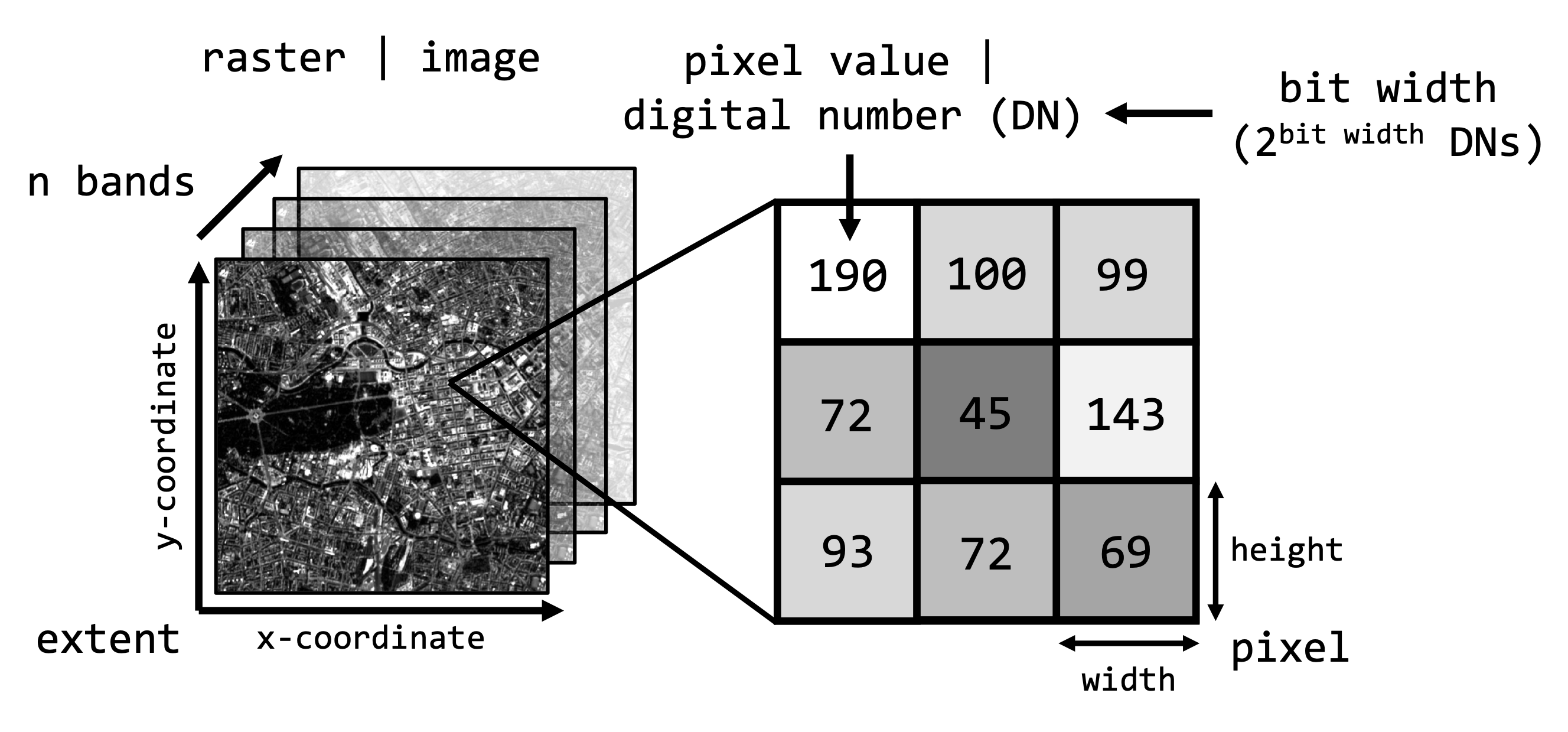
Recall the image properties from last week:
Once we have a SpatRast object in R, we can access the
properties and values of the image. Below are some terra
functions to access some of these properties and how to access
individual bands or pixel values:
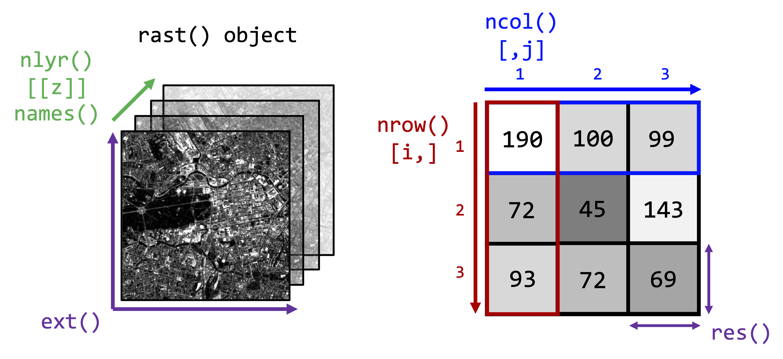
You can imagine the image as a three-dimensional array in which each
pixel has a xyz-coordinate or index which we can access using square
brackets []. For example, to retrieve the values from the
third band (here the red band) at row = 1000 and column = 500 we would
write:
# raster[[zdim / band]][ydim / row, xdim / column]
img_s2[[3]][1000, 500]
## SEN2A_BOA_20190726_RED_flt32
## 1 0.0369img_landsat[[3]][1000, 500]## RED
## 1 541Index the same xyz-index in the Landsat-8 and Sentinel-2 raster stacks. What do you notice in terms of the values returned? Why does the same xyz-index (i.e.,
[[3]][1000, 500]) in the Landsat-8 and Sentinel-2 raster
stack not point to the same geographic area?
Data types
Note how the Landsat-8 data is stored as integers (whole numbers) while the Sentinel-2 data is stored in float (decimal numbers). It is time to revisit the data types from last week.
Recall that we quantized the radiometric resolution of a sensor in bits:
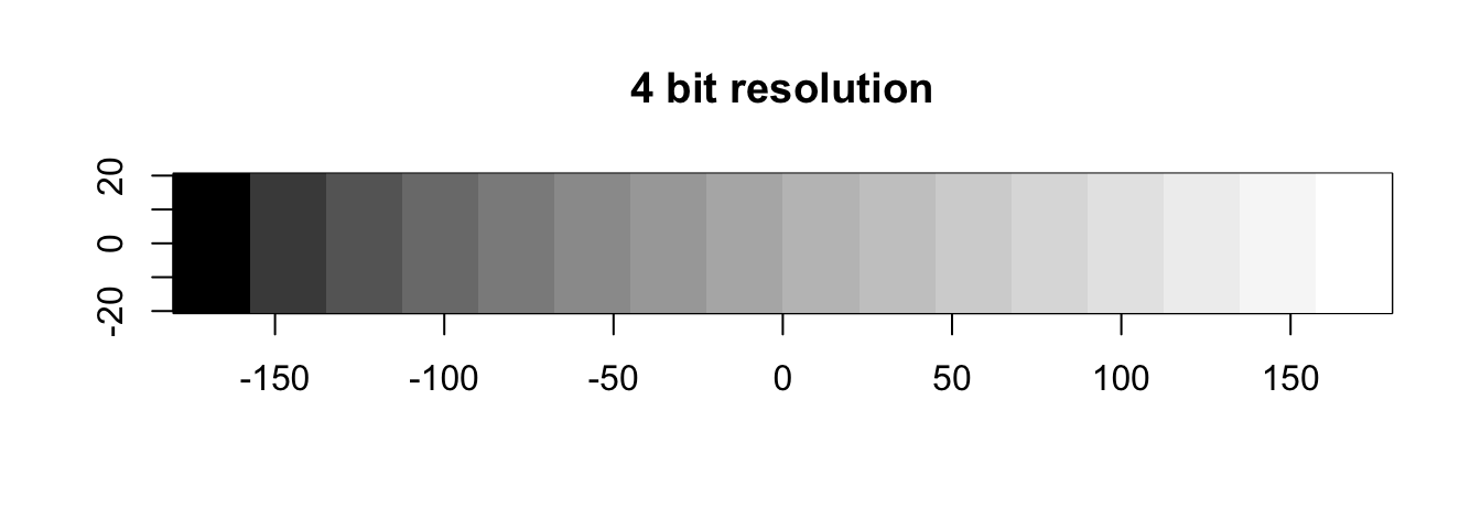
If the radiometric resolution is high, smaller and more subtle differences in reflected electromagnetic radiation can be differentiated by the sensor. The measured energy is then converted and stored as digital numbers, the pixel values in the imagery. The range of unique values that can be stored in each pixel is determined by the data type, thus the radiometric resolution greatly governs the needed data type to store the data. The unit in which the radiometric resolution and data type are measured is bits, i.e. short for binary digit. If you want, you can learn more about the binary system in the R-Basics section “Data Types”.
For now, we are only concerned with the common data types of numeric data structures:
| Data type (name) | Typical bit length | Value range | R datatype |
|---|---|---|---|
| byte / int8 | 1 byte = 8 bit | -128 to 127 (signed); 0 to 255 (unsigned) | 'INT1S'; 'INT1U' |
| int16 | 2 byte = 16 bit | -32768 to 32767 (signed); 0 to 65535 (unsigned) | 'INT2S'; 'INT2U' |
| float | 4 byte = 32 bit | -3,4e^38 to 3,4e^38, ‘single precision’; floating point number according to IEEE 754 | 'FLT4S' |
| double | 8 byte = 64 bit | -Inf to +Inf, ‘double precision’ | 'FLT8S' |
The data types byte and 16bit integer store whole numbers while float
and double store floating-point values, i.e., decimal numbers. For
example, if you wanted to store the number 3.14 as integer,
it would be in the potential range of both data types, 8bit and 16bit
(signed and unsigned). However, both types cannot store decimal places
and thus the decimal positions would be truncated, resulting in
3 as the stored value.
Now you may ask why even bother choosing another datatype than double, which covers large numbers and decimals? Well, a greater bit length (8bit vs. 32bit) also means we need to actually store this information on our data storage device, possibly without needing to, because the information we would like to store could be stored more efficiently with a smaller bit length. This is because the bit length determines the file size of the image.
Data type
determines file size The file size or memory needed to store an image can be calculated as follows:
file size = number-of-bands × number-of-columns × numbers-of-rows × bit-length
Consider what the above means for the Sentinel-2 data. Our image has the following dimensions:
dim(img_s2)## [1] 4977 6279 6The pixel values are currently stored as 32bit floating point numbers. The uncompressed filesize in megabyte is thus approx. equal to:
# n_pixels * bit width
n_pixels <- prod(dim(img_s2))
bytes <- 4  # 32 bit integer
print( paste0( "Size (Mb) 32bit: ", round( n_pixels * bytes / 1024**2, digits=2 ) ) )
## [1] "Size (Mb) 32bit: 715.27"If we can somehow change the data as 16bit integer, the file size reduces to:
# n_pixels * bit width
n_pixels <- prod(dim(img_s2))
bytes <- 2  # 16 bit integer
print( paste0( "Size (Mb) 16bit: ", round( n_pixels * bytes / 1024**2, digits=2 ) ) )
## [1] "Size (Mb) 16bit: 357.63"With growing amount of images, it is inevitably useful to think about datatypes and use tricks to store data more efficiently. Often we convert data from float (% reflectance between 0-1) to integer by simply multiplying by a constant value of e.g. 10,000, where a value of, for instance, 0.353 (35.5%) becomes 3530, allowing for an int16 data type. This way we can represent the decimal reflectance numbers as integer and save a lot of memory on our hard drives.
Raster algebra
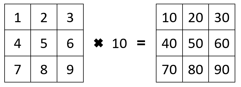
The task to save disc space gives us a good reason to learn how to change pixel values of raster objects. Recall from the R Basics section that vector/array arithmetic works element-wise:
a_vector <- c(1, 2, 3, 4, 5)
print(a_vector * 10)
## [1] 10 20 30 40 50You can add, subtract, multiply or divide a constant from every element in the array.
We can also use these operations on multiple arrays of the same size. For example multiplying two arrays together, the first element of the first array is multiplied by the first element of the second array, and so on.
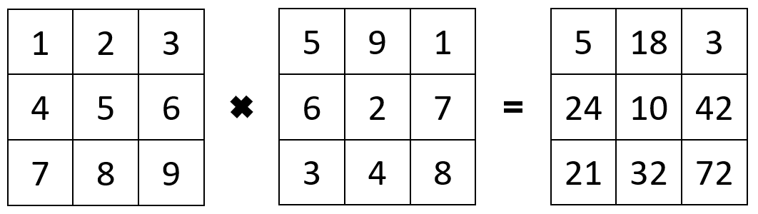
When we apply an operation on our SpatRaster, the
terra package performs the matrix operations for us in the
back, meaning operations on SpatRaster objects work
element-wise, too.
Change the pixel values of your Sentinel-2 raster stack to an integer compatible value range. First, inspect the value range of the Sentinel-2 data by using the
hist() function
on your raster stack. Second, take a look at the datatype table above
and select an appropriate datatype. We would like to use an integer, but
retain the radiometric sensitivity of the data. Third, based on the
above, select an appropriate constant scaling factor to multiply your
raster stack with. Fourth, write your raster stack to disc, explicitly
providing the needed function argument writeRaster() to use
the appropriate datatype. Last, compare the two Sentinel-2 raster stacks
(float vs. integer) in your folder in terms of their filesize.
Reprojecting and spatial subsetting
Our last basic raster handling tool for today will deal be reprojections and spatial subsetting. A common entry point for spatial analysis is the need to reproject raster data to a different coordinate reference system (CRS) or to subset the data to a specific Region Of Interest (ROI). The original extent of the image data seldom matches our ROI.
Our ROI is the city of Berlin, whose extent is stored in a rasterized
form in the file berlin_10m_epsg32633.tif.
The file contains the desired extent and coordinate reference system
(CRS) for our project.
When we compare the Coordinate Reference System
(CRS) of the Sentinel-2 image to that of the ROI image,
we notice that they are different. We thus need to reproject the
Sentinel-2 image to match the projection and grid of
berlin_10m_epsg32633.tif.
The following figure depicts a zoom-in comparing the
10x10m target grid of berlin_10m_epsg32633.tif
(red), to the 10x10m grid of your Sentinel-2 image
(grey).
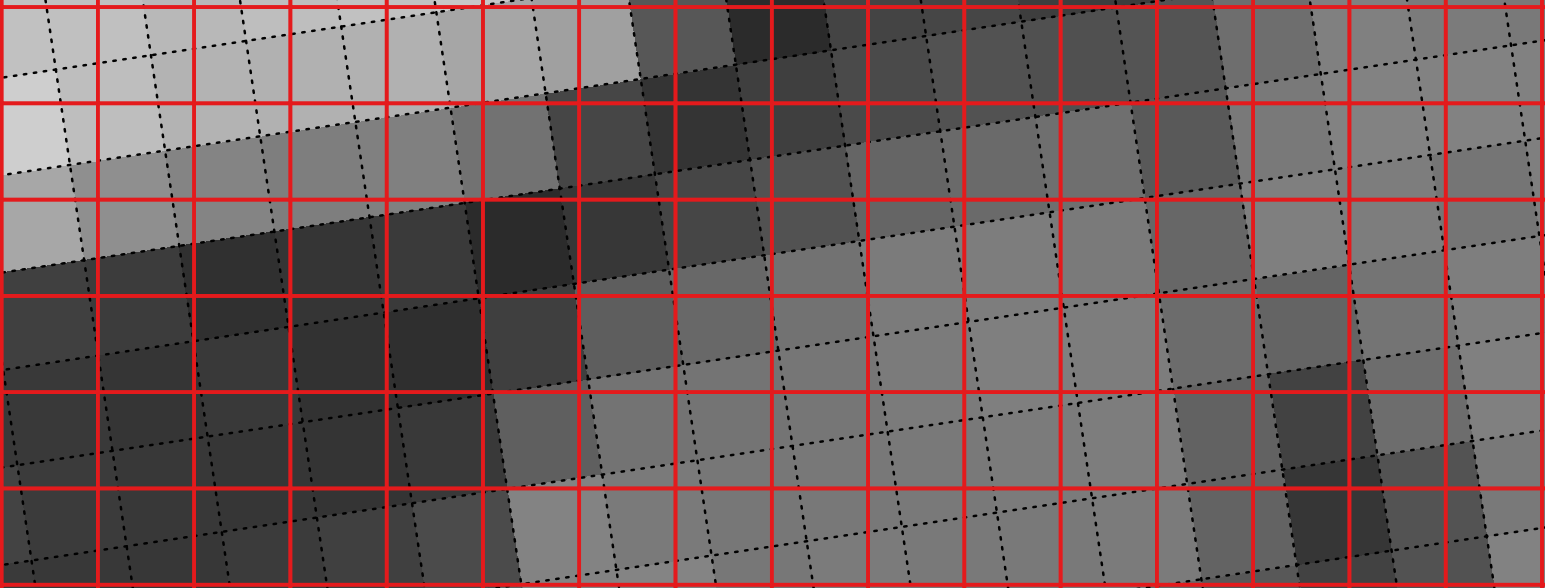
We would like to transform the Sentinel-2 onto the red grid. But since the grids obviously do not match perfectly, how do we compute the values in the new grid? In technical terms this process is called resampling. We must choose a resampling method which defines the way the values in the output raster will be computed from the input raster. The three most commonly used techniques are Nearest Neighbour, Bilinear Interpolation and Cubic Convolution:
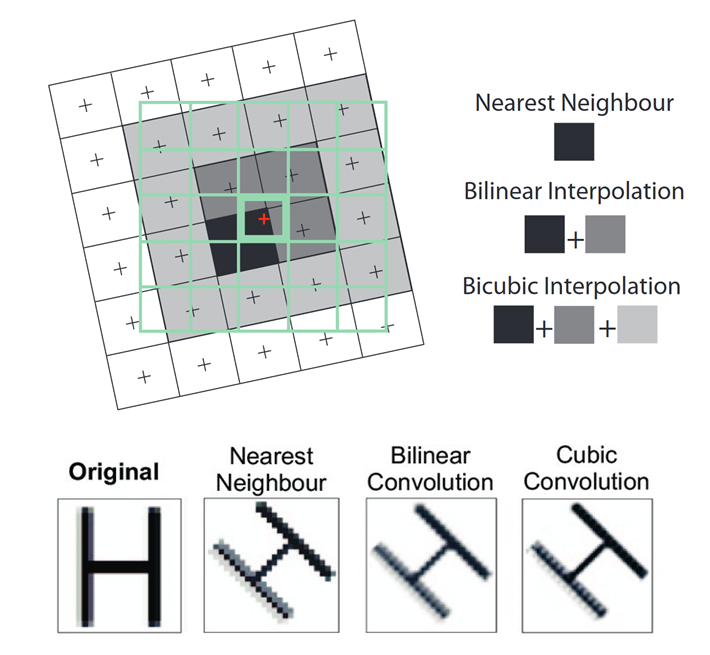
- Nearest Neighbour: The value of each cell in an output raster is calculated using the value of the nearest cell in an input raster. The original value is not altered.
- Bilinear Interpolation: The value of each cell in an output raster is calculated using the weighted average value of the nearest four cells in an input raster.
- Cubic Convolution: The value of each cell in an output raster is calculated using the weighted average value of the nearest 16 cells in an input raster.
Assignment
In today’s homework assignment you will…
- reproject the Sentinel-2 data to match the study area
- inspect the atmospheric influence by visually comparing top-of-atmosphere (TOA) vs. bottom-of-atmosphere (BOA) reflectance
- inspect the difference in the measured signal by comparing Landsat-8 with Sentinel-2 imagery from the same acquisition date
Reprojections
Reproject image
Reproject your 16bit integer Sentinel-2
image using berlin_10m_epsg32633.tif as reference image for
projection, extent and resolution. To do this, make use of terra’s
project() function. Seek the help page
(?project) and identify the correct values for the
arguments x and y. Create two separate reprojection
results, once using 'near' and once using
'cubic' for the method argument. Print your result
to console and check if the extent and dimensions match as expected.
Then, write both results to disc.
Assess results in QGIS
Compare the results for both
resampling methods in QGIS. Zoom in and out to search for
differences/patterns. Considering the above theory on resampling
methods, your visual assessment, and if necessary additional resources
online: Which method is more appropriate for the Sentinel-2 data? Can
you come up with a general rule of thumb when to use Nearest Neighbour
over Bilinear/Cubic resampling depending on the raster input? To
exemplify your argument, include at least one screenshot in your
.Rmd file using the following syntax:
{width=100%}
The signal altered by the atmosphere: TOA vs. BOA
In the lecture you have learned about the influence of the atmosphere on the measured signal. You heard that we try to eliminate the atmosphere and calculate the surface reflectance as if there was no atmosphere. Data that is not atmospherically corrected is refered to as Top-Of-Atmosphere (TOA) reflectance. Atmospherically corrected data represents surface conditions and is thus called Bottom-Of-Atmsophere (BOA).
In our case, we have worked with two different products: The Landsat-8 data is TOA reflectance, and the Sentinel-2 data is BOA reflectance.
With both datasets opened in QGIS, use the the “Identify features”
at the top-panel to right-click
selected pixels and select “Identify All”. Change the view from “Table”
to “Graph” to see the spectral profiles for both images on top of each
other.
Now select different pixels and compare the spectral profiles of the two images to each other. Identify an exemplary pixel for 1) woody vegetation (e.g. forests), 2) built-up and 3) water, and provide a screenshot for each of the profiles. For each profile then describe the general pattern of reflectance in the different wavelengths and identify the most notable differences between TOA and BOA. Based on what you learned in the lecture, explain the most prominent difference between TOA and BOA.
Submission
Document your answers to the questions above with bullet points and the help of your screenshots in your
.Rmddocument knitted to PDF.Upload your documentation as a PDF file on Moodle.
General submission notes: Submission deadline for the weekly assignment is always the following Monday at 10am. Please use the naming convention indicating session number and family name of all students in the respective team, e.g. ‘s01_surname1_surname2_surname3_surname4.pdf’. Each team member has to upload the assignment individually. Provide single file submissions, in case you have to submit multiple files, create a *.zip archive.
Copyright © 2023 Humboldt-Universität zu Berlin. Department of Geography.
![]()