Learning goals

Understanding the principles of bi-temporal change detection
Introducing case studies

Background

Change detection principles

Remote sensing provides great opportunities to observe and monitor changes on the land surface. Using satellite based images, changes over long periods of time as well as over large areas can be revealed. This section aims at providing insights into the most basic form of change detection - the bi-temporal change detection.

Bi-temporal change detection

To illustrate the procedure for bi-temporal change detection, we consider a hypothetical example of deforestation mapping. We are given two images for the same study site, one from 1999 and one from 2011.

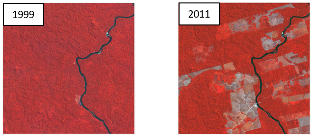
Landsat images for 1999 and 2011 in false-color visualization

For each image we want to produce a binary map showing forest / non-forest. To do so, we collect two sets of training data points: one for both classes in each image. Next, we use supervised classification techniques (e.g. Random Forest) to create one map per image. In this case we train one classification model for each image.

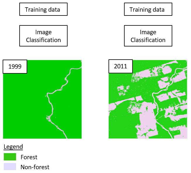
Creating binary classifications for 1999 and 2011

As a next step, we want to derive change information from the two maps. We can therefore combine the maps in order to assess class sequences for each pixel. Remember, the classes in the map correspond to numeric values, e.g. 1 (forest) and 2 (non-forest). Technically, we can thus use a simple mathematical operation to derive interpretable and unambiguous change classes, where e.g. 12 indicates forest (1) to non-forest (2) change, i.e., deforestation.

The most straightforward is to multiply the pixel values of the first image with 10 and then add the pixel values of the second image. As an example:

Stable forest (forest to forest): 1 * 10 + 1 = 11
Deforestation (forest to non-forest): 1 * 10 + 2 = 12

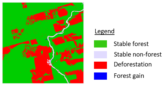
Change map showing all possible change classes

This map allows us to assess if change has occurred or not. In the binary case we can observe two types of stable sites

Stable forests: pixels with class label forest in 1999 and forest in 2011
Stable non-forests: pixels with class label non-forest in 1999 and non-forest in 2011

Also, we can observe two change classes

Deforestation: pixels with class label forest in 1999 and non-forest in 2011
Forest gain: pixels with class label non-forest in 1999 and forest in 2011

Depending on the research question at hand, researchers may want to focus on the occurrence a single change process. In this example, we want to focus on deforestation. We can then perform a reclassification of the class values in order to aggregate the change map into two classes:

Deforestation (1): the target class, only deforestation (12)
Others (2): the remaining classes: stable forest (11), stable non-forest (22), forest gain (21)

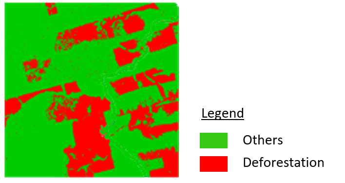
Change map showing only the target change process

The resulting binary change map can then be assessed in terms of map quality using the standard procedures of accuracy assessment. We need an independent sample for map validation. Based on this sample, we compare class labels of our map with class labels of the validation dataset. We construct a confusion matrix and calculate the typical accuracy scores: overall accuracy, user´s accuracy, producer´s accuracy as well as the corresponding errors.

Assignment

In the coming weeks, you will perform a bi-temporal change detection for a set of case studies covering different parts of the globe. Each individual case study targets at mapping one particular change process, such as deforestation, flooding, or agricultural expansion using Landsat or Sentinel-2 data. Key results will be presented in a short presentation. The schedule for the coming weeks is as follows:

18.01.2023: Introduction and initial work on the case study
25.01.2023: Continuiung the work on the case study
01.02.2023: Finalizing the case study work
15.02.2023: Presentation of key results

Objective of the work is a remote-sensing based characterization of land cover change. You will work on the case study in your breakout groups.

Introducing the case studies

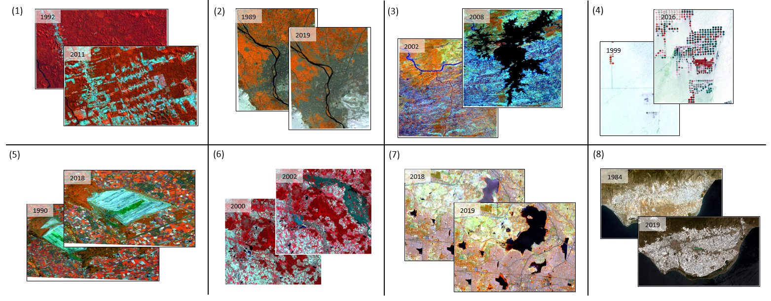
We selected eight diverse study sites, some of which relate to the time series interpretation of last week. Each site is unique in terms of the study period, the target change process, particularities of the land cover types. Each group can select one site, some sites may be selected twice.

Case nr.	Name	Location	Target process	Target class	Other class	Sensor(s)	Period
1	Deforestation	Brazil, Pará	Deforestation	Primary forest	Non-Primary forest (incl. pastures, crops, soil, shrubs, secondary forest, settlements)	Landsat 5	1999 -2011
2	Urbanization	Egypt, Kairo	Urban Growth	Urban	Non-urban	Landsat 5/8	1989 - 2019
3	Reservoir flooding	India, Indirasagar Dam	Reservoir flooding	Water	Non-Water (including seasonally flooded rice fields)	Landsat 5/7	2002 - 2008
4	Cropland expansion	Egypt, East Oweinat	Cropland expansion	Irrigated area (including the non-vegetated parts)	Non-irrigated area (desert, roads, airport, settlements etc.)	Landsat 7/8	1999 - 2016
5	Deforestation	Germany, Hambach	Deforestation	Forest	Non-Forest	Landsat4/8	1990 - 2018
6	Flooding	Germany, Elbe river	Flooding	Water	Non-Water	Landsat 7	2000 - 2002
7	Drying lakes	India, Chennai	Shrinking water extent	Water	Non-Water (including seasonally flooded rice fields)	S2	2018 - 2019
8	Greenhouse expansion	Spain, Almeria	Greenhouse expansion	Greenhouse / Other		Landsat 5/8	1984 - 2019

Materials

For every case study, we provide the necessary images and a set of reference data for validation in this folder:

Satellite images: a pair of Landsat or Sentinel-2 images for two points in time
Validation dataset: a shapefile of 100 random samples, collected with 500 m minimum distance, containing the following attributes:
- date_1: class labels for the target (1) / other (2) classes in the first point in time
- date_2: class labels for the target (1) / other (2) classes in the second point in time
- change: the combination of class labels from both points in time
- bin_change: class labels for the target change process (1) / no-change and all other change processes (2)
Study region boundaries: a polygon shapefile
Presentation slide template (PowerPoint)

Workflow

The analysis workflow can be divided in six steps and summarized graphically as follows:

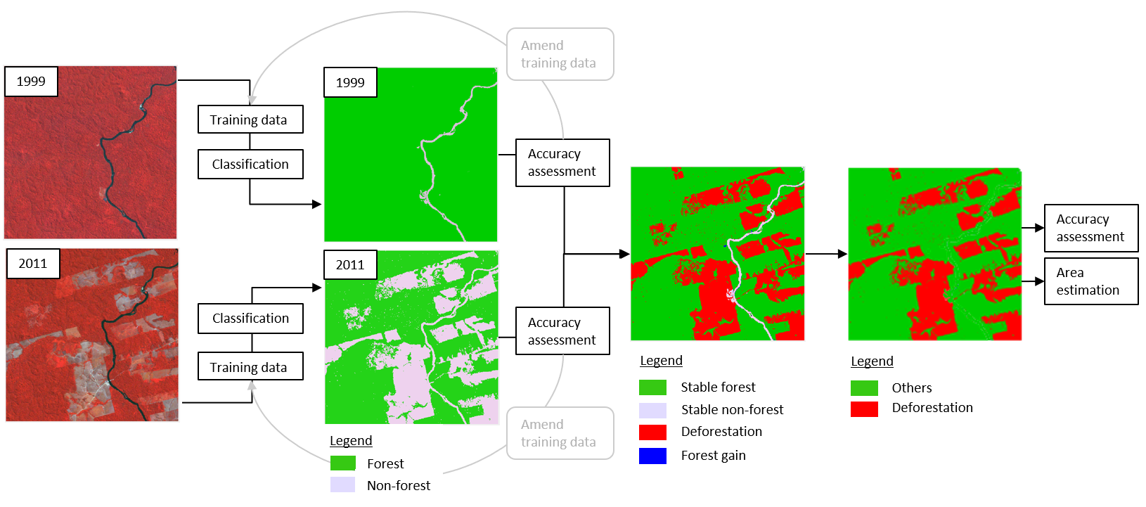
Bi-temporal change detection workflow

1) Screen data

Open both satellite images for your study region in QGIS and visualize it in a meaningful setup, considering true-color / false color representation and an appropriate contrast stretch, as learned in session 02.
Screen your study region in both time periods and get acquainted with the land cover types present in both images.
Investigate your study region in Google Earth, using recent or historic imagery. You may want to add the polygon delineating the study region. Use the Send2GE plugin to zoom to a coordinate in GooglEarth by clicking on your QGIS map canvas.

2) Collecting training data

Create a shapefile for your training data points for each time step (2 shapefiles in total) for a binary classification of your target class and the others class. It should
- have a point geometry
- match the projection (EPSG-code) corresponding to the input images
- contain one column for the class id of the respective time step. The field must be of type integer with length 2.
Collect a sufficient number of representative training points for your target class and the remainder class, as described in the table above.
Note your class ids as 1 for the target class, and 2 for the remainder class.
The General principles of training data collection communicated in session 09 apply.

3) Random Forest classification

Use the Random Forest classification algorithm to produce a binary classification for each time step. For every time step, use the respective training dataset and the input image.
Follow the procedure described in session 09.

4) Validation and improvement

Assess the quality of your binary maps visually and quantitatively based on the provided validation data.
Follow the procedures described in session 10.
If obvious and systematic errors occur, you may amend your training dataset and produce another classification.
Iterate training amendment, classification and validation until you are satisfied with the results.

5) Change Detection

Use imageMath to create a change map showing all possible (no) change classes following the procedure outlined above. Take a look at the following code template:

# Change detection with 4 classes
# Create two variables containing the classification of the first and second satellite image:
# 'classification_1' and 'classification_2' refers to your input variables

class1 = classification_1
class2 = classification_2

# Create a new variable 'change_map' and combine both classifications by multiplying 
# the pixel values of the first image with 10 and then adding the pixel values of the second image
# Note that you need to specify the output variable 'change_map' in advance

change_map = class1 * 10 + class2

Visualize the change map in QGIS
Rename the change classes in light of your target classes, e.g.
- 11 = Stable forest
- 12 = Deforestation
- 21 = Forest gain
- 22 = Stable non-forest

6) Aggregating classes

Aggregate non-relevant classes to class “others” using imageMath. Make sure your target change class is represented as value 1, the others class as value 2. For instance:
- 12 –> 1 = Deforestation
- 11, 21, 22 –> 2 = Others
Take a look at the following script on how to do a reclassification of your map:

# Reclassification of 4 change classes into 2 final change classes
# Create a new variable named 'classes'
# 'change_map' refers to your input variable (your previously calculated change map)
# with change_map[0] we are copying the first layer of your change map to a new variable 'classes'

classes = change_map[0]

# Create an empty raster using properties (size, projection, etc.) of another raster

classes_reclassified = np.zeros_like(classes)

# Fill the empty raster with the new class values
# Specify whether the class represents target change (1) or other (2) similar to the example below
# With == you are referring to a specific class, i.e. class 11 (e.g. urban to urban)
# Note that the target change class depends on the target change process in your study region,
# e.g. for urbanization you want to define 21 (non-urban to urban) as target change (1)
# for deforestation it may be 12 (forest to non forest).

classes_reclassified[classes == 21] = 1
classes_reclassified[classes == 11] = 2
classes_reclassified[classes == 12] = 2
classes_reclassified[classes == 22] = 2

7) Validating the change map

Perform an accuracy assessment of the final change map using the reference data we provided (attribute “bin_change”). The procedures for validating the change map are identical to 4)

8) Summarizing key results

Calculate absolute (e.g. hectares) or relative (percentage of study area) area estimates that describe the change process, e.g. area deforested in hectares, or how much percent of the forest hast been deforested. You can use the “Classification Statistics” tool in the EnMAP Box to assess the class statistics in your map.
Create a useful change map in QGIS that highlights your key results.
Consider basic rules of cartography concerning map layout, information, color palettes, etc.

9) Presentation

Use the presentation template to prepare a short presentation of your case study. Follow the guidelines in the template for your presentation.
Submit your presentation slides in Moodle until Monday, 13.02.23, 10:00 am.
Successful seminar participation requires that all group members must participate in the presentation. We schedule 10 minutes per group.

12. Change detection case studies