Entry into the raster data world

Before we delve into specific aspects of practical Earth Observation during the semester, we would like to give you the opportunity to warm-up your data handling skills along a small project. Our goal will be mapping the 2002 flood of the river Elbe, Germany. Although our approach to mapping the floods is going to be rather simplistic, it allows for touching upon some fundamental aspects of dealing with raster data (in R).

In order to do this, we must learn to …

… acquire data: Visit USGS’s EarthExplorer platform and query the Landsat archive
… read, write, manipulate and visualize raster data in R
… setting up a processing workflow using functions
… extract water surfaces from imagery using boolean indexing

Exercise 1: Acquisition of remotely sensed data

The Earth’s atmosphere, water, and land surfaces are being observed by a plethora of instruments constructed for varying purposes. The technical properties of these instruments vary broadly and as a result, the data retrieved from such instruments also contains diverse types of information in various data types and formats. These raw datasets often require additional processing using automated algorithms which make them useful for communities with different applications at hand. But how is the data made accessible to the users?

Public institutions such as the United States Geological Survey (USGS) and the European Space Agency (ESA) play a key role in this regard, as they currently host the most relevant platforms for Earth Observation data distribution - the USGS Earth Explorer and ESA´s Copernicus Open Access Hub. Most (but not all) of the data provided on these platforms are currently available free of charge.

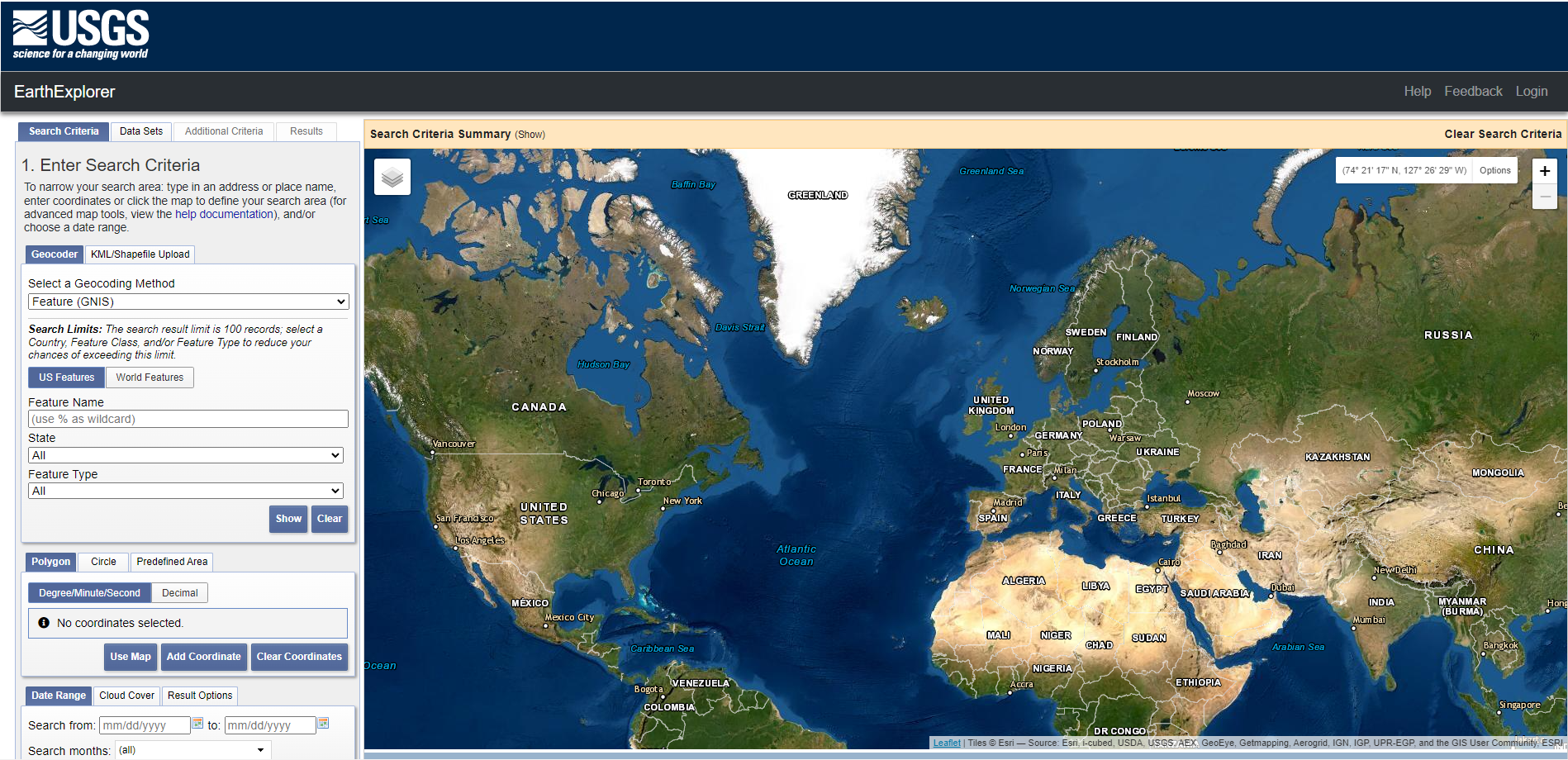
USGS EarthExplorer website

Let’s get some Landsat data: The Landsat mission comprises eight multispectral Earth observing satellites, with Landsat-1 initially launched in 1972. From the launches of Landsat-4 and Landsat-5 Thematic Mapper’s (TM) onwards, the Landsat mission featured at least six key bands in the optical domain at 30m spatial resolution: blue, green, red, nIR, SWIR1 and SWIR2:

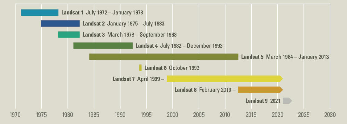
The Landsat mission timeline (Source: USGS)

Now, as mentioned above, our goal is to map the August 2002 flood of the river Elbe, Germany. We will make use of two image acquisitions for this: One before, and one during or shortly after the flooding.

Query search
Visit the USGS Earth Explorer and use the Address/Place field to navigate to Elster (Elbe), Germany (close to Wittenberg, at lat: 51.82, lon: 12.82). Switch to the ‘Data Sets’ tab and select Landsat -> Landsat Collection 2 Level-1. Tick the Landsat 7 ETM+ C2 L1 box and click on ‘Results >>’.

Filter search criteria
You´ll get several hundreds of results, so let´s narrow down the search since we are only interested in imagery until the 31st of August 2002. First, under ‘Search Criteria’, set the ‘Date Range’ to before 08/30/2002. Second, only include the summer months June, July and August in your search query. Third, adjust the ‘Cloud Cover’ threshold to only include imagery with 0% - 10% cloud cover (because we have not yet learned how to deal with clouded imagery, but we will). Last, click Results, and try to identify the ‘flood-scene’ by clicking the small image icon to visualize the data. Then, identify a ‘pre-flood’ image which has the same spatial extent and no clouds obscuring the target.

Order / download data

download the data from our repository

Exercise 2: Raster reading, metadata and writing in R

The `terra` package

The terra package offers useful classes and functions which facilitate raster data handling in R. It allows us to access file characteristics before loading data into memory, manipulate coordinate r eference systems and spatial extents. We can use it to perform raster algebra, to combine raster and vector datasets (e.g. ESRI shapefiles), or to convert raster files into matrices, which are compatible with the base functions we use to subset data, access image statistics, develop models, and much more. The terra package supersedes the older raster package developed by the same team of authors. Because raster has been around for a longer time, dependencies with some packages may still exist. But development of raster will eventually be stopped at some point. terra’s classes and functions are well described in the package documentation.

The most important classes within the package are:

SpatRaster to store raster data
SpatVector to store spatial vector data, i.e., points, lines, polygons.
SpatExtent to store information on spatial extents

There are a couple of things that the terra package does not provide. For example, collecting training and validation data are preferably done in a GIS environment (e.g. QGIS) and processing large data volumes is preferably achieved in other programming languages than R. Advanced visualization of spatial datasets can be done in R using additional packages (e.g., ggmap, tmap, mapview). We appreciate and encourage you to play around and find the visualization techniques that appeal to you the most.

Welcome to the `terra` world

Install the terra package (like any other package) as shown below. All dependencies will automatically be installed.

# Install the terra package
install.packages('terra')

# Load the package
library(terra)

Read and inspect a raster file

Navigate to one of the folders containing an unpacked Landsat image. Did you take a close look at the Landsat file naming convention? Practically, it provides some basic meta-information. For instance, LE07_L1TP_193024_20020820_20200916_02_T1 is a sequence of information on the sensor (LE07), processing level (L1TP), WRS path and row (193/024), acquisition date (20020820), processing date (20200916), collection (02), and collection tier (T1), separated by ’_’.

As you can see, the Landsat images are delivered as single-band files. To get started we want to import a single band of the Landsat-7 scene during the flood event, inspect the metadata, and learn about SpatRaster objects in terra.

The rast() function creates a SpatRaster object in R. One can create a SpatRaster from scratch, by providing a filename, or from another object. For now, we use the function to import a single band:

band4 <- rast("LE07_L1TP_193024_20020820_20200916_02_T1/LE07_L1TP_193024_20020820_20200916_02_T1_B4.TIF")
# to print the metadata of the object, simply call the object:
band4

## class       : SpatRaster 
## dimensions  : 7611, 8241, 1  (nrow, ncol, nlyr)
## resolution  : 30, 30  (x, y)
## extent      : 220185, 467415, 5615085, 5843415  (xmin, xmax, ymin, ymax)
## coord. ref. : WGS 84 / UTM zone 33N (EPSG:32633) 
## source      : LE07_L1TP_193024_20020820_20200916_02_T1_B4.TIF 
## name        : LE07_L1TP_193024_20020820_20200916_02_T1_B4

As you can see, calling/printing the object in the command line provides you an overview on some of the metadata. There are a number of basic functions that are useful in everyday use to check the metadata of a raster file. You find a quick overview about the main SpatRaster methods of terra here. Take a look and try to find a out the following:

What is the spatial resolution of the imagery (+ unit)?
How can we extract the coordinate reference system as variable from the image?
How do we rename the layers in our raster object, e.g. to ‘B4’ in our case?
How does the rast() function deal with NA-values?

Combining the single band images into a stack

Since we want to make use of more than just the information from the NIR band (band 4), the single bands should be stacked for further analyses. For stacking, all input files must have matching extents and the identical projection. For the rest of this practical, please include the f ollowing bands: blue, green, red, near infrared, shortwave infrared 1, shortwave infrared 2 (in this order). Always keep the band designations in mind, as this can cause confusion, e.g. when combining Landsat-7 and Landsat-8 data. Check the list of Landsat spectral bands for a recap:

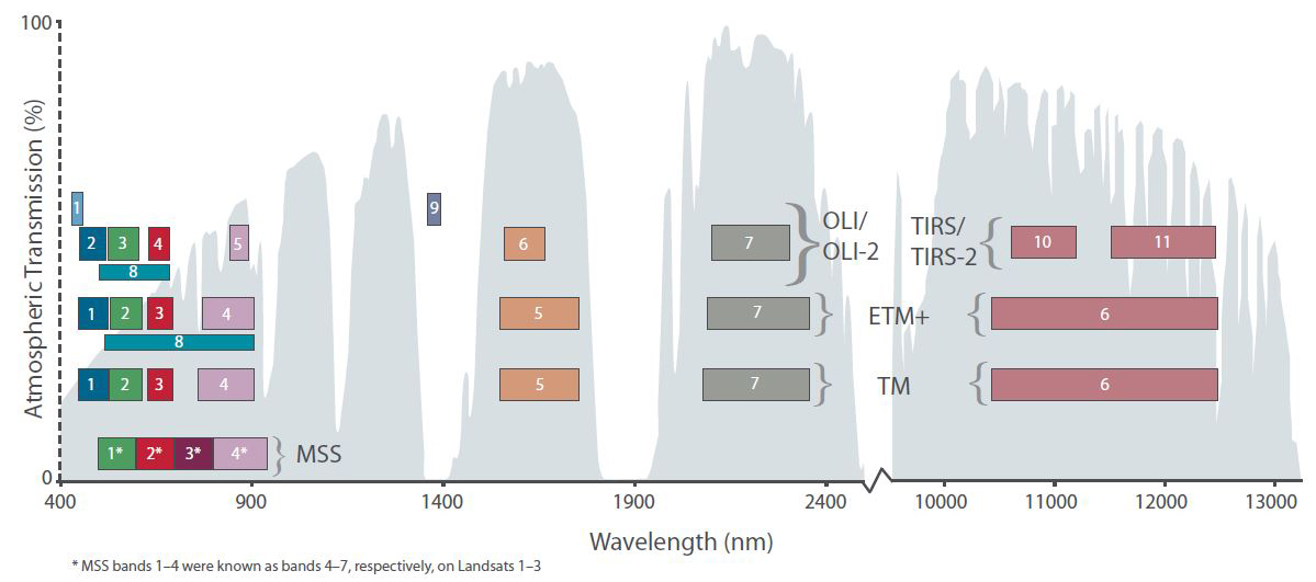
Band designations for Landsat satellites

Which bands (i.e. their number, e.g. ‘B1’) will we have to include accordingly?

Now, based on the procedure for the single band above, we could start declaring a single variable for each band…

band1 <- rast("LE07_L1TP_193024_20020820_20200916_02_T1/LE07_L1TP_193024_20020820_20200916_02_T1_B1.TIF")
band2 <- rast("LE07_L1TP_193024_20020820_20200916_02_T1/LE07_L1TP_193024_20020820_20200916_02_T1_B2.TIF")
band3 <- rast("LE07_L1TP_193024_20020820_20200916_02_T1/LE07_L1TP_193024_20020820_20200916_02_T1_B3.TIF")
# ... but wait!

That would require a lot of typing and neither would it be very reproducible (given changing filenames for any other scene). Instead, the first helper function will be list.files(). Here, this function will allow us to acquire a list of the files (as characters) in a given directory:

# apply list files to the folder of the first image
files <- list.files("LE07_L1TP_193024_20020820_20200916_02_T1")

# let's print the first 11 elements of the file list to check its elements
print(head(files, 11))

##  [1] "LE07_L1TP_193024_20020820_20200916_02_T1_ANG.txt"      
##  [2] "LE07_L1TP_193024_20020820_20200916_02_T1_B1.TIF"       
##  [3] "LE07_L1TP_193024_20020820_20200916_02_T1_B2.TIF"       
##  [4] "LE07_L1TP_193024_20020820_20200916_02_T1_B3.TIF"       
##  [5] "LE07_L1TP_193024_20020820_20200916_02_T1_B4.TIF"       
##  [6] "LE07_L1TP_193024_20020820_20200916_02_T1_B5.TIF"       
##  [7] "LE07_L1TP_193024_20020820_20200916_02_T1_B6_VCID_1.TIF"
##  [8] "LE07_L1TP_193024_20020820_20200916_02_T1_B6_VCID_2.TIF"
##  [9] "LE07_L1TP_193024_20020820_20200916_02_T1_B7.TIF"       
## [10] "LE07_L1TP_193024_20020820_20200916_02_T1_B8.TIF"       
## [11] "LE07_L1TP_193024_20020820_20200916_02_T1_GCP.txt"

As you can see, the folder contains more than just the .tif-files we need. Now, list.files() can do a lot more.

Use the internal help of R …

?list.files

… to understand the additional arguments pattern, recursive, and full.names of the list.files() function. The pattern argument allows for quite some detailed filtering and may take some time to get accustomed to. Therefore, use the following pattern - "*B[1-7]*.TIF$" - and try to make sense of it by looking up regular expression under the help section of pattern in ?list.files.

Last, create a raster stack object using list.files() and terra::rast(). Using your insights from earlier, also rename the bands of your raster stack to "blue", "green", "red", "nir", "sw1", "sw2".

# apply list files to the folder of the first image
img_files <- list.files(, pattern = , full.names = )
stack <- rast(img_files)

print(stack)

## class       : SpatRaster 
## dimensions  : 7611, 8241, 6  (nrow, ncol, nlyr)
## resolution  : 30, 30  (x, y)
## extent      : 220185, 467415, 5615085, 5843415  (xmin, xmax, ymin, ymax)
## coord. ref. : WGS 84 / UTM zone 33N (EPSG:32633) 
## sources     : LE07_L1TP_193024_20020820_20200916_02_T1_B1.TIF  
##               LE07_L1TP_193024_20020820_20200916_02_T1_B2.TIF  
##               LE07_L1TP_193024_20020820_20200916_02_T1_B3.TIF  
##               ... and 3 more source(s)
## names       : blue, green, red, nir, sw1, sw2

Now that we have our raster stack combined and renamed, let´s write it to disc using the writeRaster function of terra:

writeRaster(stack, "")

Exercise 3 - Manipulating raster data

Plotting raster image using R

We can plot a SpatRaster object using the built-in plot function in R, resulting in each band plotted separately:

plot(stack)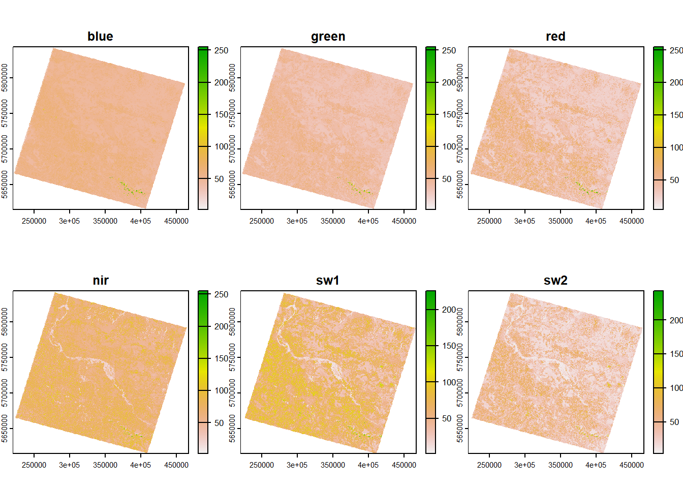

terra provides us a plotRGB() function, which comes in handy to plot a true-color (R: red, G: green, B: blue) or false-cover (e.g., R: SW1, G: NIR, B: red) representation of an image. We just need to make sure to properly consider the order of bands in our stack (1 = blue, 2 = green, 3 = red, 4 = nIR, 5 = swIR 1, 6 = swIR 2) in relation to our computer screen´s color channels (1 = red, 2 = green, 3 = blue).

plotRGB(stack, r=3, g=2, b=1, stretch="linear")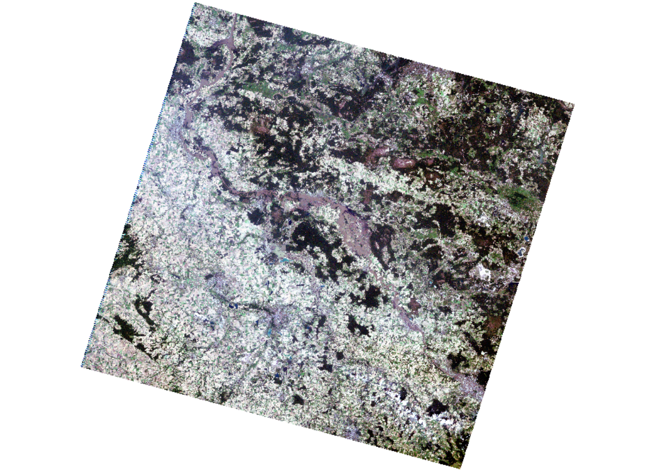

Plot a false-colour representation of your image where photosynthetic active vegetation is displayed in red tones.

Spatial subsetting

Currently, we are working on the entire image scene, yet we are provided with a Region of Interest (ROI) (ROI.gpkg) which we may use to spatially subset or crop/clip our image dataset.

# read in vector file using terra::vect
roi <- vect("ROI.gpkg")

# plot image and ROI
plot(stack$nir)
plot(roi, add=T)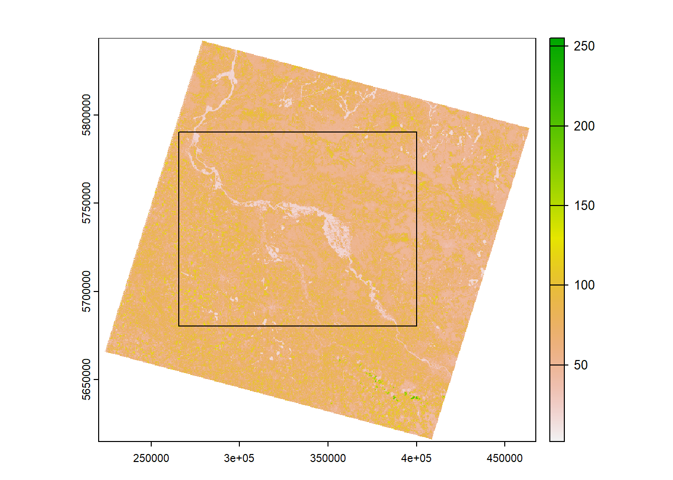

Take a look at ?crop and subset your image stack to the Region Of Interest.

stack <- crop()

Raster Algebra: Converting DN to reflectance

Take another look at the actual values stored in our raster stack, e.g. by plotting a single band:

plot(stack$blue)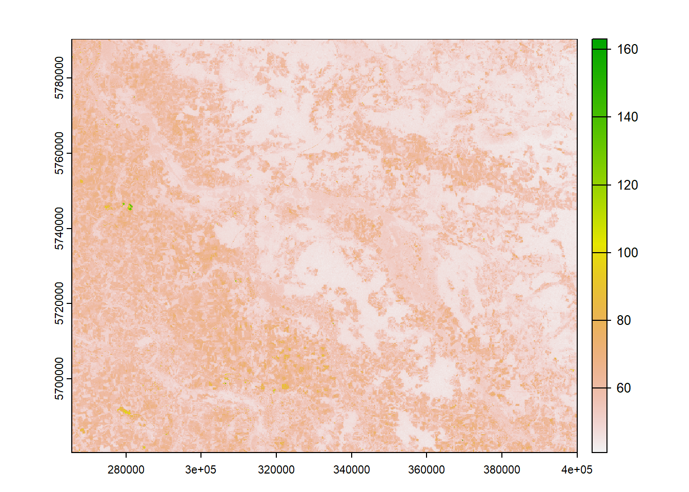

Remote sensing sensors translate measured radiance to Digital Numbers (DNs) to store the acquired energy as digital data. DNs express the amount of radiance in relation to sensor-specific calibration coefficients. As DNs are dependent on the sensor calibration, identical measurements yield differing DNs across sensors. Since DNs are just used to store the data, they are physically not meaningful and need to be converted to radiance or reflectance values using the sensor-specific calibration coefficients.

The (re-)scaling involves a simple linear transformation:

\[Reflectance = \beta_{1} * DN + \beta_{0}\],

where DN are the Digital Numbers (i.e. pixel values), and $\beta_{1}$ and $\beta_{0}$ are the band-specific calibration coefficients. The calibration coefficients for Landsat-7 are found in the metadata .txt file (LE07_L1TP_193024_20020820_20200916_02_T1_MTL.txt). We will dig deeper into the topic in Session 2 during the actual course, allowing you to fully understand every detail. For now, what is important to us is that we would like our data to be interpretable reflectance instead of DNs and in order to get there, we need to convert the DNs using the formula and associated coefficients. Luckily, we have a function which extracts us the coefficients from the metadata file automatically only by inputting the scene directory, see:

# get conversion factors
get_conv_val <- function(inp_dir){
  mtl <- list.files(inp_dir, pattern='MTL.txt$', full.names=T)
  mtl_txt <- read.delim(mtl, sep = '=', stringsAsFactors = F, header = FALSE) 
  names(mtl_txt) <- c("VAR", "VAL")  # add header
  REFLECTANCE_MULT_BAND <- as.numeric(mtl_txt[grep("REFLECTANCE_MULT_BAND_[1-7]", 
                                                   mtl_txt$VAR),][,2])
  REFLECTANCE_ADD_BAND <- as.numeric(mtl_txt[grep("REFLECTANCE_ADD_BAND_[1-7]", 
                                                   mtl_txt$VAR),][,2])
  return(list(REFLECTANCE_MULT_BAND, REFLECTANCE_ADD_BAND))
}

coeffs <- get_conv_val("LE07_L1TP_193024_20020820_20200916_02_T1")
print(coeffs)

## [[1]]
## [1] 0.0018653 0.0020966 0.0019879 0.0029110 0.0027755 0.0026288
## 
## [[2]]
## [1] -0.011660 -0.013188 -0.012534 -0.018227 -0.017290 -0.016465

beta1 <- coeffs[[1]]  # multiplicative beta1 is 1st entry in list
beta0 <- coeffs[[2]]  # additive beta0 is 2nd entry

Now that we have the formula and the coefficients, all we need to understand is how to apply it to each pixel value of our raster stack. Luckily, that is rather straight forward:

As you might remember, images are numerically represented as matrices. Matrices are 2-dimensional arrays with a specified number of rows and columns. All columns in a matrix must have the same data type (e.g., numeric, character) and must be of equal length.

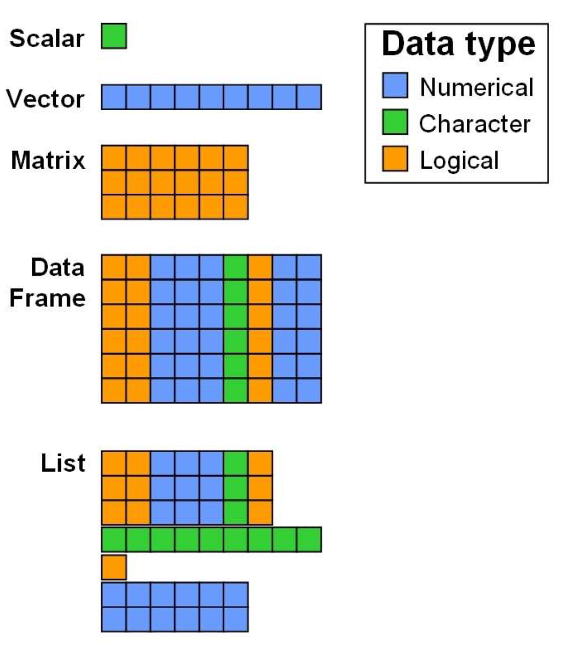
Data Structures in R (from Zimmermann & Steinmann 2006)

Mathematical operations can be used to manipulate arrays. You can add, subtract, multiply or divide a constant from every element in the array.

# Create an array of one 4x3 matrix
a <- array(data=c(1:9), dim=c(4,3,1)) 

a2 <- a * 10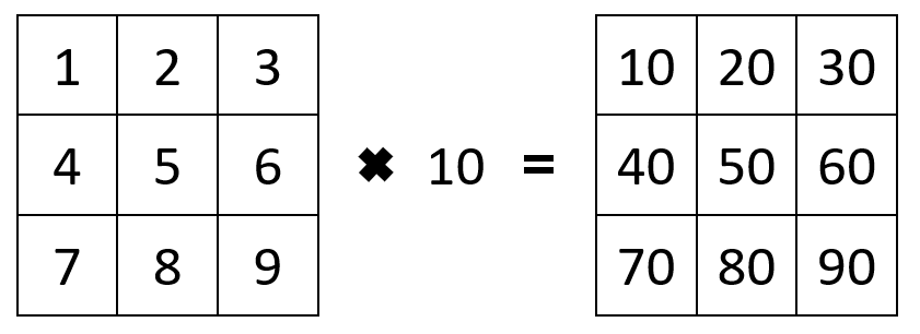

An entire array can be scaled by multiplying it with a constant

We can also use these operations on multiple arrays of the same size. This array arithmetic works element-wise. For example multiplying two arrays together, the first element of the first array is multiplied by the first element of the second array, and so on.

# Create two arrays, each of one 4x3 matrices
a1 <- array(data=c(1:9), dim=c(4,3,1)) 
a2 <- array(data=c(1:9), dim=c(4,3,1)) 

a3 <- a1 * a2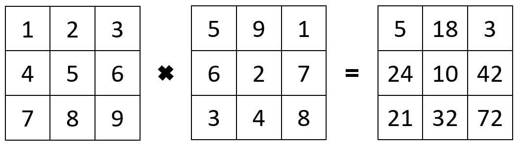

You can multiply two images with each other in a pixel-wise manner

When we apply an operation on our SpatRaster, the terra package performs the matrix operations for us in the back, meaning operations on SpatRaster() objects work element-wise, too.

Convert your image, consisting of DNs, to physically meaningful reflectance values by applying the above equation and coefficient vectors on your stack variable.

stack_reflectance <-

Verify your operation by plotting a single band and checking the value range.

Exercise 4: Workflow using functions

Wrap your processing in one continuous workflow

One of the many advantages of using a languange like R, instead of a GIS environment, is that you are able to easily apply a workflow to a great amount of data repeatedly. In case of remote sensing, we often want to automatically process hundreds or thousands of images. R offers you a variety of flow control structures to wrap you processing steps into generalized workflows (if-else, loops, functions). For this course, we want you to apply the same processing we applied to the first Landsat-7 image to the second Landsat-7 image using a function. Rememember: It is crucial to understand the properties of our data (e.g. NA-values, extents, data types) to be able to apply the same procedures to data from different locations or times. In this case, we do not have to worry about that.

First, a little recap on functions from the R basic´s subpage:

Generally, a function is a set of statements organized together to perform a specific task. Using functions greatly enhances code structure as it improves the clarity and readability of your script.

Function arguments are provided in round () brackets. Between {} stands the function body which contains the collection of statements. return() is used to define the output of a function.

An example of a function could be calculating the NDVI for a given pair of reflectance values in the red and near-infrared region of the spectrum:

# Function to calculate the NDVI
calc_ndvi <- function(red, nir, scale_factor=1){
  ndvi <- (nir-red)/(nir+red)
  # set outer bounds to NA
  ndvi[ndvi > 1 | ndvi < -1] <- NA
  return(ndvi*scale_factor)
}


ndvi <- calc_ndvi(stack$red, stack$nir)
print(ndvi)
plot(ndvi)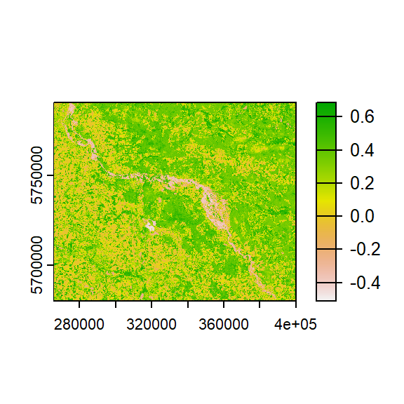

## class       : SpatRaster 
## dimensions  : 3664, 4483, 1  (nrow, ncol, nlyr)
## resolution  : 30, 30  (x, y)
## extent      : 265575, 400065, 5680425, 5790345  (xmin, xmax, ymin, ymax)
## coord. ref. : WGS 84 / UTM zone 33N (EPSG:32633) 
## source      : memory 
## name        :        nir 
## min value   : -0.5945946 
## max value   :  0.7055215

Here, red and nir are obligatory arguments that the user has to specify while scale_factor is optional as such that it has a default value which may or may not be altered.

Now back to our processing workflow

Implement a function which takes as input an input directory containing single band Landsat-7 images to be processed, and optionally allows for spatially subsetting your data (= two function arguments: input directory and ROI).

listing the desired band-files
reading them into a raster object (stack)
Optional argument: spatially subsetting the data to ROI (hint: take a look here https://stackoverflow.com/questions/28370249/correct-way-to-specifiy-optional-arguments-in-r-functions)
scaling the DNs to reflectance values
calculating the NDVI
stacking the multispectral bands and the NDVI and return the resulting object

Click here to view one version for such a function

preprocess_l7 <- function(input_dir, roi=NULL){
  
  # list single band files
  img_files <- list.files(input_dir, pattern = "*B[1-7]*.TIF$",
                          full.names = T)
  img <- rast(img_files)
  names(img) <- c("blue", "green", "red", "nir", "sw1", "sw2")
  
  # crop to ROI?
  if(!is.null(roi)){
    img <- crop(img, roi)
  }
  
  # convert DNs to rho
  coeffs <- get_conv_val(input_dir)
  img <- img * coeffs[[1]] + coeffs[[2]]
  
  # calc and add NDVI
  ndvi <- calc_ndvi(img$red, img$nir)
  names(ndvi) <- "ndvi"
  img <- c(img, ndvi)
  
  return(img)
}

# use function (variable roi must be read first)
# pre-flood image
img_pre <- preprocess_l7("LE07_L1TP_193024_20000814_20200917_02_T1", roi)
plot(img_pre)
# post-flood
img_post <- preprocess_l7("LE07_L1TP_193024_20020820_20200916_02_T1", roi)
plot(img_post)

Exercise 5: Flood mapping

Take a look at the following plot:

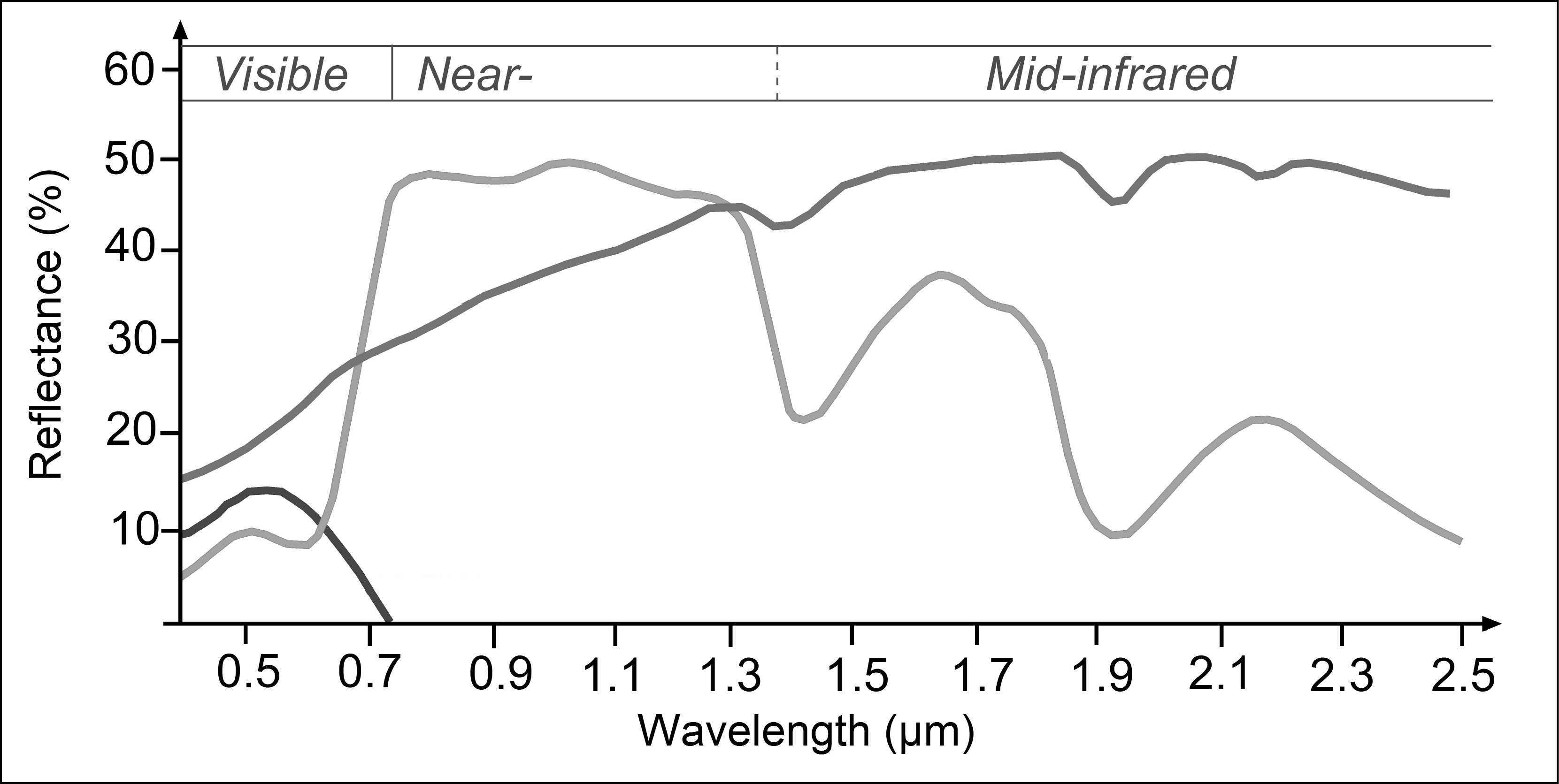
Spectral signatures of three major surface types

To which major three surface types do the spectral signatures in the plot above correspond to?
With our goal of extracting water for both images, which wavelength region would you choose to get good results? Which threshold would you choose?
Think of the above calculated NDVI - could this index be of help?

Thresholding & Logical operations

Based on your insights from above, you identified a threshold for the index/band and now want to extract to classify your images into water and non-water. We can make use of indexing and logical operators to achieve this. Consider the following: We came up with a first threshold to separate water from non-water by filtering for pixels that exhibit negative NDVI values. To create a new raster image containing 1 or TRUE where NDVI < 0, we simply type:

# all of the following result in the same 
img1_water <- stack$ndvi < 0  # only works if band is actually named "NDVI"!
img1_water <- stack[[7]] < 0  # if NDVI is 7th band in stack

If this looks unfamiliar, please have another look at the R Basics, specifically “Indexing”.

We can also combine multiple logical statements, for example two conditions:

# all of the following result in the same 
img1_water <- stack$ndvi < 0 & stack$sw2 < 0.05 # NDVI < 0 AND SW2 < 5%

Combining binary maps into final map

If we extracted the water surfaces for both images and thus hold a raster object for both dates with 1 = water; 0 = non-water, we can simply add both images together to get a new raster with our final assessment:

# all of the following result in the same 
flood <- water1 + water2
plot(flood)

Based on visual assessment, how satisfied are you with the result? What could be potential problems of such a simple approach?