Vegetation indices and data transformations

Learning goals

Calculate vegetation indices (NDVI, EVI) on image time series
Understand Tasseled Cap transformations

Background

Spectral behavior of vegetation

Vegetation exhibits a distinct spectral reflectance appearance due to its chemical composition and its physiognomy/structure. Non-photosynthetically active vegetation (NPV) (e.g. dry litter, stems) differ considerably from photosynthetically active vegetation (PV) across different wavelength regions. Reflectance of PV is determined by different factors in the VIS, NIR and SWIR region of the electromagnetic spectrum:

VIS – leaf pigments - In the visible bands the reflectance is relatively low as the majority of light is absorbed by the leaf pigments. Chlorophyll strongly absorbs energy in the blue and red wavelengths and reflects (a little) more in the green parts of the spectrum. This is why healthy vegetation appears green to the human eye.
NIR – cell structure - For healthy vegetation, the reflectance is much higher in the near infrared (NIR) region than in the visible region due to the cellular structure of the leaves, specifically the spongy mesophyll. Therefore healthy vegetation can be easily identified by the high NIR reflectance and generally low visible reflectance.
SWIR – water content - The reflectance in the shortwave infrared (SWIR) wavelengths is related to the water content of the vegetation and its structure. Water has strong absorption around 1.45, 1.95 and 2.50 µm. Outside of these absorption bands in the SWIR region, reflectance of leaves generally increases when water content in the leaf decreases.

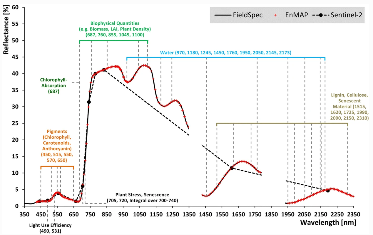
Vegetation spectrum in hyperespctral (ASD FieldSpec4, EnMAP) and multispectral (Sentinel-2) resolution as well as characterictic spectral features caused by various constituents and processes (absorption lines shown as grey dashed lines) (Source: Hank et al. 2018).

Vegetation indices

Vegetation indices make use of this particular reflectance signal. Most commonly known and applied are the Normalized Difference Vegetation Index (NDVI) and the Enhanced Vegetation Index (EVI).

Normalized Difference Vegetation Index (NDVI)

The NDVI relates the difference between the NIR and red reflectance to their sum.

\[NDVI = \frac{ρ_{NIR} - ρ_{RED}}{ρ_{NIR} + ρ_{RED}}\]

For instance, a red reflectance of 10% and a NIR reflectance of 50% results in a value of 0.666. The full NDVI response surface looks as follows:

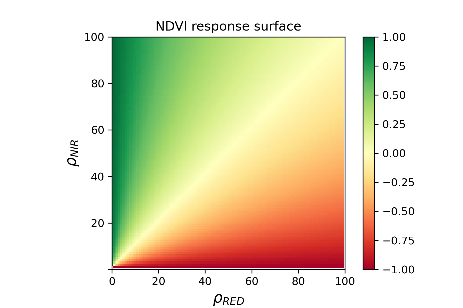
The NDVI is not a physical measure, yet a proxy for photosynthetic activity, leaf vitality, density and canopy structure. Because of its relation to vegetation density and structure, the NDVI may be used to estimate biophysical parameters such as the Leaf Area Index (LAI).

Enhanced Vegetation Index (EVI)

The EVI often has a better correlation with biomass than NDVI, specifically in vegetation canopies with low and high LAI values.

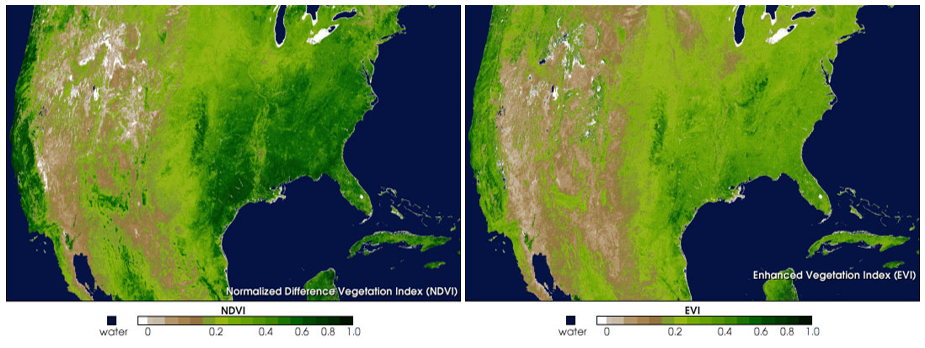
NDVI and EVI from MODIS image composites (5-20 March 2000). Source: http://earthobservatory.nasa.gov/

\[EVI = G * \frac{ρ_{NIR} - ρ_{RED}}{ρ_{NIR} + (C_{1} * ρ_{RED} - C_{2} * ρ_{BLU}) + L}\]

The correction factors for calculating the EVI from Landsat data are:

\(G = 2.5\)
\(C_{1} = 6\)
\(C_{2} = 7.5\)
\(L = 1\).

The EVI aims at reducing saturation effects which are common for NDVI. It includes a correction for soil background effects (L) to improve sensitivity for low density vegetation canopies. It is less sensitive to high aerosol loads in the atmosphere, since the additional coefficients (\(C_{1}\) and \(C_{2}\)) steer the aerosol resistance term, and the visible blue reflectance (\(ρ_{BLU}\)) is used to correct for scattering that also affects the visible red.

Indices enhance differences in reflectance to highlight certain features. Vegetation indices have the advantage of being simple, but the disadvantage of disregarding information of the spectral feature space. Linear transformations, such as the Tasseled Cap Transformation, can help to overcome this limitation.

Data transformations

Data transformations apply some function \(f\) to transform an input \(x\) to an output \(f(x)\). Often this is motivated by emphasizing certain information in the data (keeping the valuable variance) and simultaneously reducing the dimensionality. For example, Principal Component Analysis (PCA) projects an input \(x\) onto a new set of uncorrelated variables (orthogonal axes in the feature space) which preserve and amplify most of the variance in the data. From this set of components, we may choose a subset to retain most of the original variance, while simultaneously increasing interpretability and reducing dimensionality.

In the remote sensing context, one such common linear transformation is called the Tasseled Cap Transformation (TC) which already comes with a prespecified focus on certain information regarding spectral brightness, greenness and wetness.

Tasseled Cap Transformation

The Tasseled Cap Transformation (TC) is a linear transformation of the spectral bands. It was first presented in 1976 by R.J. Kauth and G.S. Thomas of Environmental Research Institute of Michigan in an article titled “The Tasseled Cap – A Graphic Description of the Spectral-Temporal Development of Agricultural Crops as Seen by Landsat.” The TC was thus developed for analyzing agricultural lands with Landsat MSS data. The name “Tasseled Cap” was chosen because the of the shape of phenological trajectories of crops in the nIR ~ red feature space.

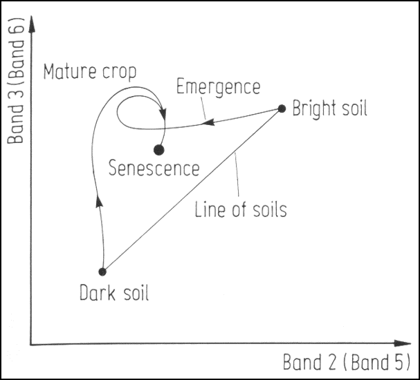
Crop phenological trajectories in near infrared ~ red featurespace. Band numbers relate to Landsat MSS bands, where band 3 (6) is the near infrared and band 2 (5) is the red band.

We can observe these trajectories by producing near infrared ~ red scatterplots for different points in time.

Animated scatterplot of 10,000 locations of an agricultural system in southeastern Turkey in near infrared ~ red featurespace, observed within the course of one year (2015).

The concept was further developed for the use with other sensors, including Landsat TM, ETM+ and OLI. It is still widely used for different remote sensing applications, especially in the context of agriculture and forestry. When analyzing the results of TC, we mostly look at three components called Brightness, Greenness, and Wetness:

Tasseled Cap Brightness (TCB): the axis along the line of soils, indicating soil brightness.
Tasseled Cap Greenness (TCG): the axis perpendicular to the soil line, emphasizes near infrared and hence vegetation.
Tasseled Cap Wetness (TCW): emphasizes shortwave infrared and is thereby related to water content.

Assignment

We provide (among other datasets for the coming sessions) the following datasets in this week’s repository:

Preprocessed Landsat-7 and Landsat-8 surface reflectance time series from 2014 to 2016 (“/imagery/time-series”)
Vector-based forestry reference information (“/vector/BDL_stand-species_EPSG3035.gpkg”)
Vector-based of Landsat 30m pixel grid (“/vector/landsat_30m_grid.gpkg/.kml”)

Today’s goal is to (1) retrieve NDVI and EVI from the VIS-NIR-SWIR Landsat time series (TC already provided to save processing time), (2) sample reference pixels for different forest types (see next subpage) and then (3) visualize the index/TC time series for the different forest types in order to assess class separability.

1) Time series data

Before we start with computing any indices, let us first screen the available time series. The data was processed using Framework for Operational Radiometric Correction for Environmental monitoring (FORCE), which is “an all-in-one processing engine for medium-resolution Earth Observation image archives” developed by David Frantz. The data provided was rigorously processed from level-1 to level-2 data by masking clouds, cloud shadows and snow or ice, correcting radiometric effects including atmospheric, topographic, BRDF and adjacency effect correction.

The imagery is provided separately for each spectral band with the following naming convention (e.g., the blue band):

2014-2016_001-365_HL_TSA_LNDLG_BLU_TSS

It provides us with the year range (2014-2016), day-of-years (001-365), the product level (HL, higher level), the FORCE submodule used for processing (TSA, time series analysis), the sensor ID (LNDLG, landsat legacy), the band/index/feature (BLU, blue band) and product type (TSS, time series stack). We thus look at a Landsat image stack of the blue band between 2014 and 2016 for all days of the years. When we open the data in QGIS or read into R we can identify that each unique observation can be differentiated by the band names (20140106_LND07, 20140113_LND07, …, 20161221_LND08). Note that R puts an X before the names (e.g., X20161221_LND08) because the string starts with a numerical value and not a character.

2) Compute vegetation indices

Calculate the NDVI and EVI time series

Remember (and as described under the section R basics -> Matrices and Arrays) that R arithmetic works element-by-element, which means we can calculate the NDVI and EVI using the time series stacks of the associated bands directly (since they are of the same length, i.e. number of bands). Read the needed BOA time-series stacks (TSS) in R and calculate NDVI as well as EVI. The correction factors for calculating the EVI from Landsat data are:

\(G = 2.5\)
\(C1 = 6\)
\(C2 = 7.5\)
\(L = 1\).

Note: The reflectance values in our datasets were saved as integer, specifically as INT2S data type. This is more efficient than saving decimal values (such as reflectance, range 0-1) in floating point data types. To do this, the data was scaled by a constant of 10,000 before writing to disc. Accordingly, a reflectance value of e.g. 0.24766 is now stored as 2476.6 and when cast to INT2S truncated to 2476. S Such a scaling approach is commonly applied and you should consider making use of this, too.

For our planned calculations, this will not make a difference when computing the NDVI. However, for the EVI the additive coefficient \(L\) must be scaled by 10,000 accordingly. Consequently, when computing the EVI from our integer Landsat time series, set \(L = 10000\).

While the computation is ongoing, please have a look at section “3) Tasseled Cap calculation” below and familiarize yourself with the time series data in QGIS. To visualize the time series at specific points in time use the virtual raster stack which combines all the time series stacks into a single virtual file "\imagery\time-series\2014-2016-4D-TSS.vrt". For instance, make a false-colour RGB composite of TCB-TCG-TCW on the 19th of July 2015. Can you identify how the surface types are coloured differently? Small note: The data is cloud mask and therefore not a gap-free time series; To find dates with almost perfect clear conditions, use the single band representation and scroll through the bands before selecting all three bands in the virtual file.

Once NDVI and EVI are calculated, prepare the stacks for export:

Make sure the data is properly scaled to be exported as INT2S
You could keep the naming convention of the image files, e.g. 2014-2016_001-365_HL_TSA_LNDLG_NDV_TSS for the NDVI stack

3) Tasseled Cap calculation (in theory)

Similarily, we could now derive the Tasseled Cap transformations using the coefficients derived by Crist (1985):

tcc <- matrix(c( 0.2043,  0.4158,  0.5524, 0.5741,  0.3124,  0.2303, 
                -0.1603, -0.2819, -0.4934, 0.7940, -0.0002, -0.1446,
                 0.0315,  0.2021,  0.3102, 0.1594, -0.6806, -0.6109), 
                dimnames = list(c('blue', 'green', 'red', 'nIR', 'swIR1', 'swIR2'), c('brightness', 'greenness', 'wetness')),
                ncol = 3)

print(tcc)

##       brightness greenness wetness
## blue      0.2043   -0.1603  0.0315
## green     0.4158   -0.2819  0.2021
## red       0.5524   -0.4934  0.3102
## nIR       0.5741    0.7940  0.1594
## swIR1     0.3124   -0.0002 -0.6806
## swIR2     0.2303   -0.1446 -0.6109

We already provide you the transformations ("/imagery/time-series") to save computational time. To calculate the transformation for the entire time series we would need more RAM or apply some tricks with tedious saving and loading in between.) The corresponding layers are:

2014-2016_001-365_HL_TSA_LNDLG_TCB_TSS -> brightness
2014-2016_001-365_HL_TSA_LNDLG_TCG_TSS -> greenness
2014-2016_001-365_HL_TSA_LNDLG_TCW_TSS -> wetness