Machine learning classification
Learning goals
- Understanding fundamentals of the Random Forest classification algorithm
- Conduct sensitivity analyses to parameterize the classification model
- Produce a forest type map for the Carpathian study region
Background
Our goal for today will be to derive a continuous forest type map for the study area in the Carpathians. The last sessions we have created features from our level-2 time series, identified representative pixels to retrieve training data and created gap-free higher level image composites and metrics. Now we want to create models that learn the spectral-temporal distribution of the four land cover classes and are able to predict the respective labels into space.
Since we use training data to build classification models, we are working in the realm of supervised learning. The chosen algorithm uses the labeled training data (e.g. image spectra and associated land cover classes) to estimate model parameters that best separate the data into their respective classes. Once this is done, we may use the trained model to estimate the appropriate class label for each pixel in the entire (unlabeled) image and thus, for example, derive a map of land cover classes.
This session focuses specifically on the Random Forest (RF) algorithm (Breimann 2001) and its implementation in R. Before we dive into the practical model building and prediction process, let us take a look at the basic principles of RFs.
“Forest”: RFs are an ensemble of self-learning decision trees (DTs). Each decision tree consists of a large number of nodes, which - starting from the root node - split into child nodes and finally leaf nodes based on binary (true | false) rules. The sequential binary branching creates the tree-like structure. Building multiple decision trees - metaphorically speaking - make up the forest. The idea behind the ensemble component of RFs is that many weak learners can come to one strong decision (i.e., a strong ensemble model).
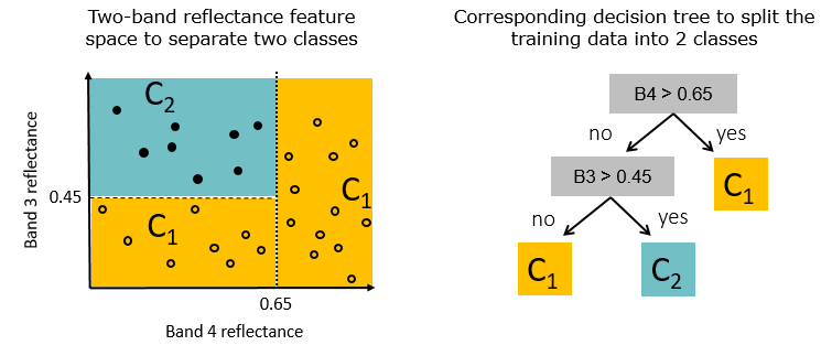
Exemplary illustration of a two-dimensional feature space, divided by binary thresholds (left), as well as the corresponding decision tree (right).
“Random”: RFs have two layers of randomness. First, they use bootstrapping (random sampling with replacement) on the pool of training data for growing the individual decision trees. Second, to create each binary node/split, RFs only consider a random subset of the features to find the best feature-threshold combination.
How a self-learning decision tree grows
Self-learning decision trees (DTs) use the concept of entropy to identify the “best split” for separating the data into two groups. Sequentially, the splitting leads to a subdivision of the data until the groups are homogeneous, i.e. the final class labels can be determined. In order to find the best split, the self-learning DTs calculate all feature-threshold combinations and choose the split that minimizes the heterogeneity of the resulting datasets. To measure heterogeneity of a dataset (or impurity, randomness, disorder), RFs often deploy the Gini impurity index (\(G_{d}\)), defined as follows:
\[G_{d} = \sum_{k=1}^{K} p_{k} (1-p_{k}) \]
where \(p_{k}\) represents the proportion of observations belonging to class \(k\) (or the probability of a datapoint belonging to class \(k\)) in dataset \(d\). The Gini index takes on small values if \(p_{k}\) is close to one for a specific class. Since we retrieve \(G_{d}\) for each of the two subdivided datasets, \(G\) for the entire split is the combined measure of \(G_{1}\) and \(G_{2}\). To account for different sizes of the two datasets, \(G_{d}\) of each sub-dataset is weighted according to its number of observations \(n_d\):.
\[G = \frac{n_1}{n_1 + n_2} G_{1} + \frac{n_2}{n_1 + n_2} G_{2}\]
In order to find the best split at each node, all feature-threshold combinations are evaluated and the one with the smallest \(G\) is selected as final split.
Randomness
If RFs were trained on the identical training data pool and were to consider all available features at each split, the decision trees would end up highly correlated. This is because DTs are sensitive to the specific dataset they are trained on and can overfit to the training data up to a degree of zero training error but with high variation when predicting on unseen data (keyword: bias-variance trade-off). To build a model that also generalises well to unseen data, RFs deploy randomness and ensembling:
Bagging - short for bootstrap aggregating - means that each DTs is build using a random sample with replacement (= bootstrap), creating random variation between the trees since they are not trained on the identical training instances. The aggregation happens at the end of creating the forest when the final class label is determined by the majority vote (average in regression) from all trees. It can be proven that this technique reduces the variance of the model (changes in model predictions on different data, from which individual DTs suffer) while keeping the low bias of the DTs (accurate predictions, difference prediction from observation).
Random feature selection for each node - the algorithm draws a random subset of features at each node, from which it identifies the split (feature and value) that produces the most homogeneous sub-groups of training data. This contributes greatly to reducing the correlation among trees. The user controls for the number of features which should be considered at each split (via the
mtryhyperparameter in the R implementation of RFs). Decreasing the number of variables tried at each split de-correlates the structure of the trees.
Prediction
The RF classifier predicts the class label for a given data point
through the majority vote of all individual trees (RF regression often
uses the mean of the values). A given data point passing through the
individual trees may receive different labels from the respective trees.
For instance, consider we have 500 trees: it may be labeled as class
1 by 280 trees, class 2 by 130 trees, class
3 by 75 trees and class 4 by 15 trees. Based
on the majority vote logic (“wisdom of crowds”), the data point will be
assigned the final class label 1.
It can be useful to analyze the information on the voting distribution in more detail. For instance, users can access the class-wise number of votes and standardize them into a probability. In the above example, we can say that
| Class | Votes | Prob |
|---|---|---|
| 1 | 280 | 0.56 |
| 2 | 130 | 0.26 |
| 3 | 75 | 0.15 |
| 4 | 15 | 0.03 |
| Total | 500 | 1.00 |
Again, low entropy can indicate “greater certainty” of the classifier. Accordingly, extracting and visualizing RF probabilities spatially can give a continuous indication on where the classifier may be more or less “certain” with its predicted label. This can be interpreted in terms of the agreement of the randomly grown trees in the specific model setup and may guide, for instance the collection of additional training data for further improving the model.
The out-of-bag error
RFs have another great feature: the out-of-bag (OOB) error. Remember: Each DT is built using a bootstrapped sample of the original training data pool. After growing each tree, the left-out samples (i.e. not used for training of this particular tree) can be classified in a test run to retrieve an estimate on expected model performance on unseen data. As we use bootstrapping, on average approx. \(\frac{2}{3}\) of the original samples are used in each tree, leaving \(\frac{1}{3}\) for testing. For instance, consider 8 left-out samples, of which 2 are wrongly and 6 are correctly classified. The OOB error will be 2/8 = 0.25. This simple measure of model performance can be useful to parameterize the classification model. We can for instance test various combinations of input features or training datasets and track how the model behaves.
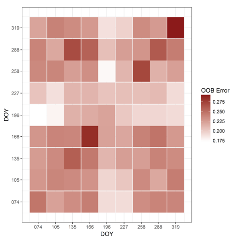
Grid representation of the out-of-bag classification error for various combinations of two input composites with different target days of the year.
Model building
The user defines the number of decision trees in the forest (e.g. via
the ntrees parameter in the R implementation). Once
ntree decision trees are built, we have a readily
applicable rule-set to classify each pixel in our image. Every tree
produces one “vote” regarding the final class outcome and the majority
of votes determines the final class label for each pixel.
Hyperparameters
- such as mtryand ntree for instance - differ
from model parameters in that they are not learned from the
data but most be specified prior to learning. Some of them can be tuned
automatically to optimize the learning process. The multitude of
different algorithms differ in their “tunability” and the Random Forest
algorithm can be considered an almost out-of-the-box working method,
largely insensitive to parameterization.
Besides ntree, the number of variables considered at
each split mtry is considered to have the greatest imapect
on model performance. Both, however, can be easily determined, making
tuning almost unnecessary. Here´s how to make informed decisions on
ntree and mtry:
ntree
Because of the random nature of the model and the weak law of large
numbers, the error of the model generally decreases as
ntree increases (because it decreases the variance error).
It will reach a point where the error rate stabilizes (converges) and
adding more trees only decreases computing performance.
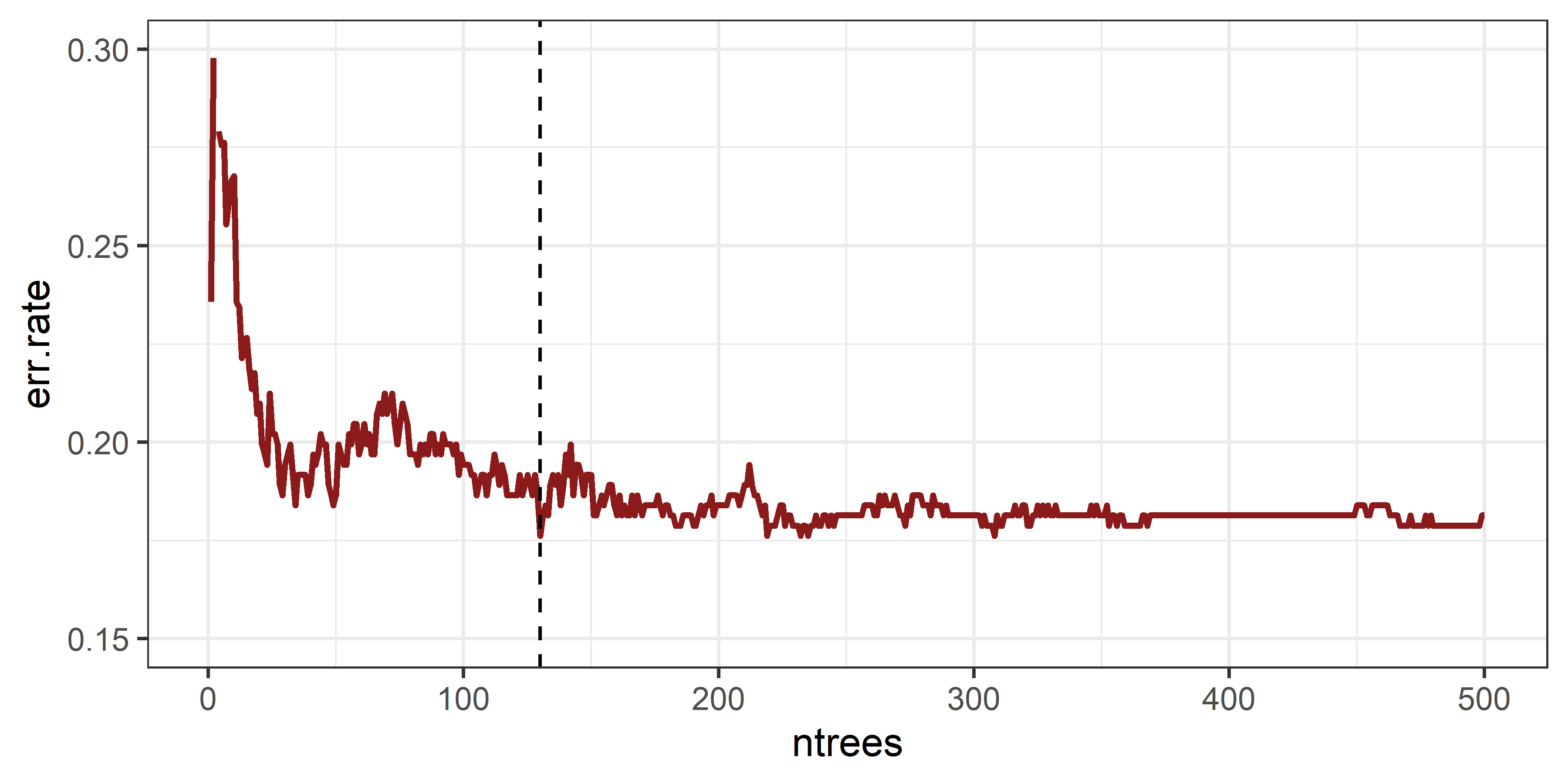
Determining the value for ntree at the absolute minimum
error rate may be intuitive at first. However, if we determine the
optimal ntree by minimizing the err.rate, we
may not look at the true point of convergence, in the below graph for
instance we may choose ntree of 130. However, there is
still a lot of variation that is noise and there is only a stabilization
after around 300 trees are grown. This number can vary depending on the
input features, training data, and complexity of the problem - there are
stochastic processes involved after all.
Due to the randomness, variability occurs between models. We
therefore recommend to verify your choice of ntrees by
looking at multiple model runs as shown below.
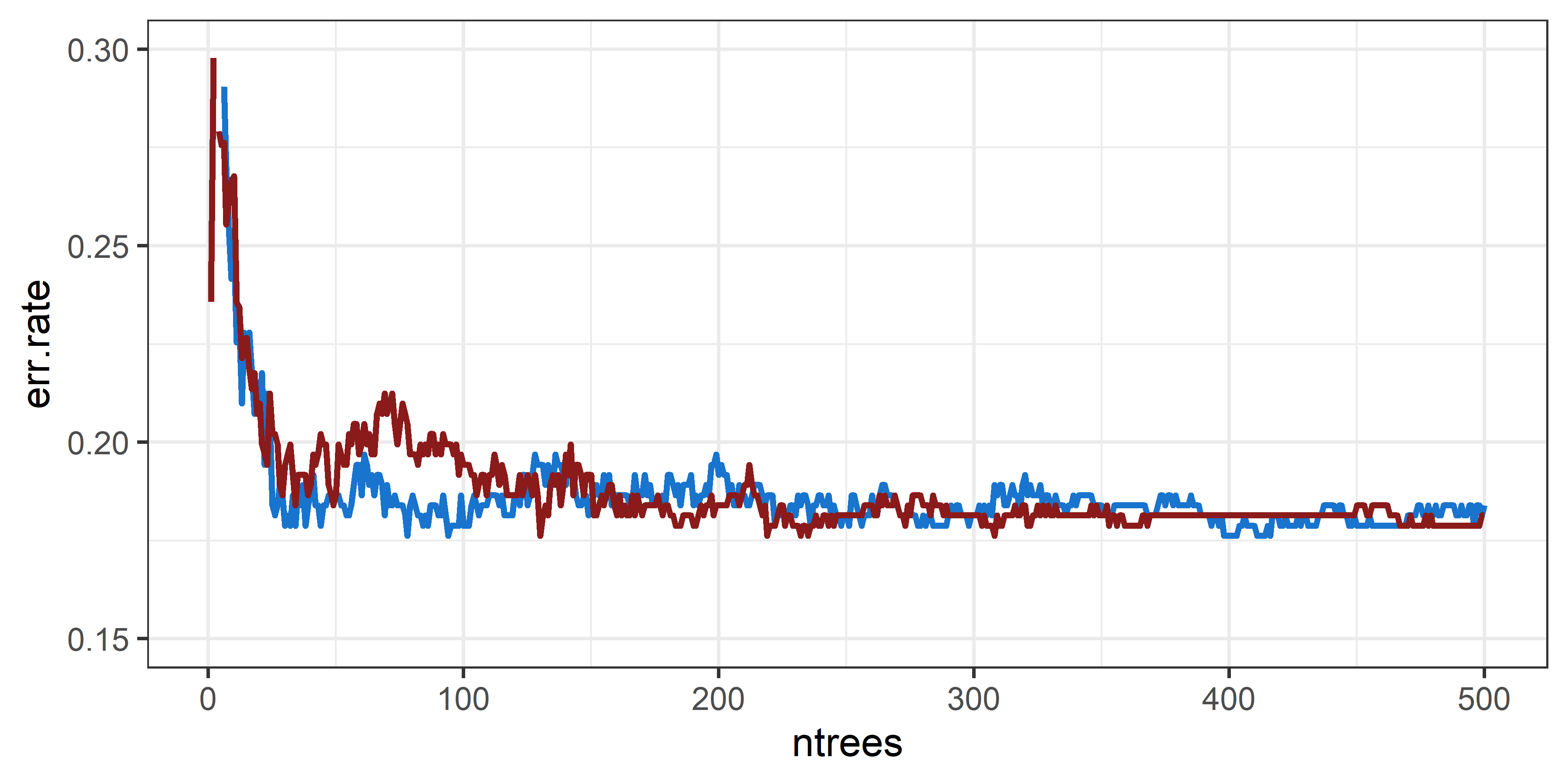
The bottom line is: tuning the number of trees is unnecessary.
Instead, set the number of trees to a large, computationally feasible
number by comparing the point of convergence across multiple model runs.
A widely used default of 500 trees can be a valid
choice.
mtry
We could optimize mtry - the number of variables
considered at each split. Setting mtry too large can lead
to overfitting because the trees are not IID
(Independent and Identically
Distributed) - they become very similar.
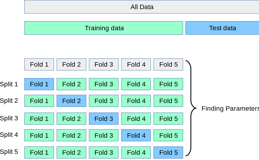
A common technique for hyperparameter tuning in general is k-fold cross-validation (CV). Using k-fold CV, The initial training dataset is split into k-partitions (= folds) where - iteratively - all folds but one are used to train the model and the withheld fold is used to validate the prediction. To minimize the variance between multiple model runs, the prediction for a certain hyper-parameter configuration is repeated k-times for k-folds of the training data to estimate the average expected error.
We can thereby identify the optimal value of mtry using
an automated grid search, which will test a user-defined set of values
for mtry and perform k iterations of model training,
prediction, and validation. Please take a look at the advanced
assignment if you are interested in exploring this further.
Back to RFs: Tuning mtry using k-fold CV is generally a
valid option, however, again RFs work very well with setting
mtry to \(\sqrt{p}\),
i.e. the square root of the number of features \(p\). This is also the default value of the
RF implementation in R.
Variable importances & partial dependence plots
Next, RF allows us to investigate which features (e.g. spectral bands) were most useful for our classification problem. Variable importance measures for each individual feature can be expressed either as mean decrease in Gini (how much “better” can we split the data based on this feature) or mean increase in accuracy (how much does the out-of-bag error increase when the feature is left out of the model). It is important to note that these variable importances should be interpreted cautiously, as they are always strongly dependent on the input feature space and the associated collinearity structure as well as the training data used. Still, the variable importance of a hypothetical model might reveal, for instance, that the swIR 1 reflectance at DOY 196 is an important feature in this model.
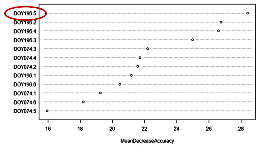
Mean decrease in accuracy (increase in OOB error) caused by the features included in the classification model.
In a next step, we can use partial dependence plots (PDPs) to further investigate the relationship between individual features and the probability of class occurrence. We can try to interpret this graph and assess relationships between individual features and our classes of interest. In the below example, the probability of occurrence for the deciduous forest class is high in the upper range of swIR 1 reflectance (above 13%), while for the coniferous forest class it is high in the lower range of swIR 1 reflectance (10% and less).
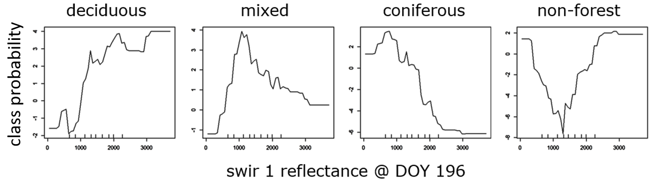
Change in class probability across the value range of the swIR 1 reflectance at DOY 196.
While generating meaningful insights is somewhat tricky with reflectance values, we could also imagine including, e.g., a digital elevation model into the RF model to learn about the probability of class occurrence across elevation gradients. An additional read on PDPs with illustrative examples can be found here.
Bottom line
Summing it up, there are a few key advantages of the RF algorithm, which make it popular in data science and remote sensing. RFs are easy to understand, computationally efficient, parameterization is straightforward, and their predictive performance is often very good. It provides quick insights into expected model performance via the out-of-bag error and allows for investigating variable importance measures and partial dependence plots.
Last, there is no single best optimization/ machine learning algorithm that can be determined a priori. It is problem specific and comparirng various models can be beneficial (keyword: “no free lunch theorem” if you are interested).
Assignment
In this assignment, we will deal with image classification using the
Random Forest algorithm, as implemented in the randomForest
package. Specifically, we will use your training data and your
pixel-based composites from the last assignments to map forest types in
the Western Beskids. We will assess the performance of multiple
classification models through the out-of-bag error and investigate
variable importances.
1) Training a Random Forest model
Our primary goal for today is to produce a forest type map. Secondary, we want to compare the suitability of the created BAPs and STMs from last session and assess which higher level image product or specifically which features might be ideal for the problem at hand. Accordingly, we are going to build multiple models and compare them using the internal model performance assessment of RFs - the OOB.
- Prepare your input data for subsequent model building.
Load the vector file containing your training data points using
terra::vect(). Next, create arast()-stack of 1) your two (or more) BAPs, 2) your seasonal STMs from last session and 3) all available datasets, i.e. all your BAPs, STMs and the STMs provided by us (covering the entire study period)For each of the three feature-sets, use
extract()to create adata.framewith training points as rows, and class labels (classID) as well as the features (bands) of your image stack as columns. Make sure that that you remove the metadata flags such as day of year and year from the PBCs (since they are not meaningful predictors)As we want to train a classifier (and not a regressor), the
randomForest()function expects the dependent variable to be of type factor. Useas.factor()for conversion of theclassIDcolumn. Like most models, the RF algorithm cannot deal with missing data (NA). Remove potentialNAsfrom thedata.frame(if there are any at all in the image)
-
Build the three
randomForest models: 1) Selected BAPs
model_bap, 2) selected STMs model_stm, 3) all
data model_all.
Train a
randomForest()classification model with the firstdata.framecreated in the prior step. Make sure to include only useful predictors. For now, setntree = 750and leavemtryto the default (\(= \sqrt{n_features}\)).Repeat the RF training procedure and produce additional model objects from the other dataframes.
2) Investigating model performance
The RF model objects contain a wealth of information on the model parameters and performance.
-
Assess the out-of-bag (OOB) error estimates of the trained models by
inspecting the
err.rate attribute of your model objects.
Answer the following questions:
Which model has the lowest OOB error? How large is the difference between the best and second best model in terms of overall accuracy?
How does the OOB behave when increasing the number of trees in your model (
ntree)? You can access the OOB per number of trees viaerr.rate. Use this information to determine a suitable maximum value forntree. From a model’s predictive performancentreecannot be too high, only the computational performance will decrease. The aim is to find the spot where the error rate stabilizes (converges) and adding more trees would no longer improve accuracy.In the model with the lowest OOB error, which of the four classes has the highest OOB error?
-
Create a second model using the merged
dataset from your fellow students. Does it perform better or worse?
Why do you think this is the case? What is potentially problematic with
this approach?
3) Feature selection
The above three models are likely to exhibit very different
predictive performance according to the OOB error. For most of you,
model_bap and model_stm are likely to perform
poorer than model_all. The constrained set of features
simply does not contain as much explainatory variance as found in the
full set of features. However, the full set of features is in turn
likely to contain a lot of redundant information (collinearity) and is
rather large, impacting model training and prediction performance.
Ideally, we would choose only the most important features for our
classification problem to reduce model complexity.
The caret package provides a simple to use
implementation of Recursive Feature Elimination (RFE).
RFE identifies the optimal amount of features through as backward
feature selection process: First, RFE builds an initial model using all
available features and calculates the importance each feature
contributes ( e.g. variable importance from RF algorithm). This allows
for iteratively ranking the importance and removing the least important
features. Finally, we can determine the feature set at at which adding
less important features does not add significantly to model predictive
performance.
Let’s see how this works using caret. First, we define
the control function which specifies the algorithm (rfFuncs
for Random Forest), the method to evaluate each model run
("repeatedcv") as well as the associated repeats and folds
of the cross-validation:
control_rfe = rfeControl(functions = rfFuncs,
                         method = "repeatedcv",
                         repeats = 5,
                         number = 5)
Next, we can already run RFE by specifying our predictors
(x), target variable (y) and control function.
The argument sizes allows us to specify the number of
features we would like to test. Here we use 1 to 5, 15, 20, …:
result_rfe = rfe(x = df_train[feat_names],
                 y = df_train$classID,
                 sizes = c(1:10, 15, 20, 25, 30, 40, 50, 60),
                 rfeControl = control_rfe)
print() and plot() your RFE result. Dexcribe
how the curve behaves and what this implies. You can retrieve the
selected set of features using predictors(result_rfe).
Build your final model using only the selected features.
4) Classification
Perform a classification of the image stack using the
terra::predict() function. Write the resulting map to disk
in GTiff format. When doing so, choose the appropriate
datatype argument. Inspect your result in QGIS and visually
identify well classified regions and classes, as well as potential
misclassifications. Does this match your expectations when assessing the
OOB error rates?
Next, calculate class probabilities for each pixel and use them to further guide your assessment of map quality. Remember: Since RFs are ensemble of single DTs, the probability of class association can be calculated by the number of votes for each class divided by the total number of trees.
### Run predict() to store RF probabilities for class 1-4
rfp <- terra::predict(img, rf_full, type = "prob", index=c(1:4))
names(rfp) <- c("p_deciduous", "p_mixed", "p_evergreen", "p_nonforest")

### Scale probabilities to integer values 0-100 and write to disk
writeRaster(rfp*100, "imagery/RF_prob.tif", datatype="INT1S", overwrite=T)-
Why and how could the probability layer be valuable for improving
another iteration of our models?
-
Now use the
predict() function to create a classified map,
using your best performing RF as the model object. Note that you now
have to delete the type=prob argument to obtain labels
instead of probabilities. Write the result to disk and evaluate the
classification in QGIS.
Voluntary: Grid-search hyperparameter tuning
The e1071 package offers automated parameter
optimization for several classification algorithms. The
tune.randomForest() function for instance allows you to
optimize the Random Forest hyperparameter mtry. Run the
below code to check, whether the tuning of mtry improves
your error rate substantially.
library(e1071)

# Define accuracy from 5-fold cross-validation as optimization measure
cv <- tune.control(cross = 5)

# Use tune.randomForest to assess the optimal combination of ntree and mtry
rf_tune <- tune.randomForest(classID~., data = train.df, ntree=750, mtry=c(2:10), tunecontrol = cv)

# Store the best model in a new object for further use
rf_best <- rf_tune$best.model

# Is the parametrization and/or different from your previous model?
print(rf_best)
Voluntary advanced assignment: Support-Vector Machines (SVMs)
Support-Vector Machines (SVMs) are another form of supervised
learning algorithms often used with remote sensing datasets. If you are
curious how the SVM approach would deal with the same classification
problem, feel free to run a test. SVMs are sensitive to parametrization,
and the parametrization is not as intuitive as it is for the RF
classifier. Luckily we can also optimize parameter settings based on a
grid search using tune.svm(). Read the SVM
vignette for further information.
SVMs can be highly flexible algorithms due to their use of
sub-functions known as kernels. Several kernels are available in the
e1071 SVM implementation (Radial Basis Function (RBF),
Sigmoid, Polynomial, Linear). Let´s stick to the RBF kernel (default
setting), as it has been showing good performance in a variety of
settings. Feel free to read the scikit-learn
tutorial on the role of the parameters \(C\) and \(\gamma\) in the RBF SVM.
The RBF kernel has the advantage of requiring the specification of
only one parameter \(\gamma\)
(gamma). Next, we have to define the parameter \(C\) (cost), which defines the
tradeoff between training error and model complexity. The authors of the
SVM implementation suggest to try a range between small and large values
for C. Below, you find a code example following the suggestions in the
scikit-learn tutorial.
library(e1071)

# Define accuracy from 5-fold cross-validation as optimization measure
cv <- tune.control(cross = 5)

# Use tune.svm() for a grid search of the gamma and cost parameters
svm_tune <- tune.svm(classID~., data = train.df, kernel = 'radial', gamma = 10^(-3:3), cost = 10^(-3:3), tunecontrol = cv)

# Store the best model in a new object
svm_best <- svm_tune$best.model

# Which parameters performed best?
print(svm_best$gamma)
print(svm_best$cost)
Now use the predict() function to classify a map as
above, using svm.best as the model object. Write the result
to disk and compare the RF and the SVM classification in QGIS.
Reading materials
In the next session, we would like to discuss the following paper:
FAO (2016): Map Accuracy Assessment and Area Estimation - A Practical Guide
The paper is outlines best practice guidelines for accuracy assessment and area estimation in the context of land change maps. Please read the paper thoroughly, make sure you understand the basic ideas behind it and write down questions for the next session. Also, answer the following broad questions:
- Why is a stratified sampling advised?
- How can we determine how many samples are needed for accuracy assessment?
- What is the difference of populating an error matrix with \(p_{ij}\) instead of \(n_{ij}\)?
- How can we derive unbiased area estimates?
Please take a look at the Excel sheet provided here. Use this table to improve your understanding of the area adjusted accuracy assessment. You can manipulate values in the confusion matrix / class proportions and trace the formulas which link these values with the resulting class-specific and overall accuracies as well as the area estimates.
We also highly reccommend you read Olofsson et al. (2014): Good practices for estimating area and assessing accuracy of land change, which documents the state-of-the-art for accuracy assessment and area estimation in the context of land change maps.
Copyright © 2020 Humboldt-Universität zu Berlin. Department of Geography.
![]()