Multi-temporal change detection

Learning goals

Combine what you’ve learned so far to develop a supervised change classification workflow
Map forest dynamics in the Southern Brazilian Amazon
Generate map-based estimates of forest loss and gain in the study region

Background

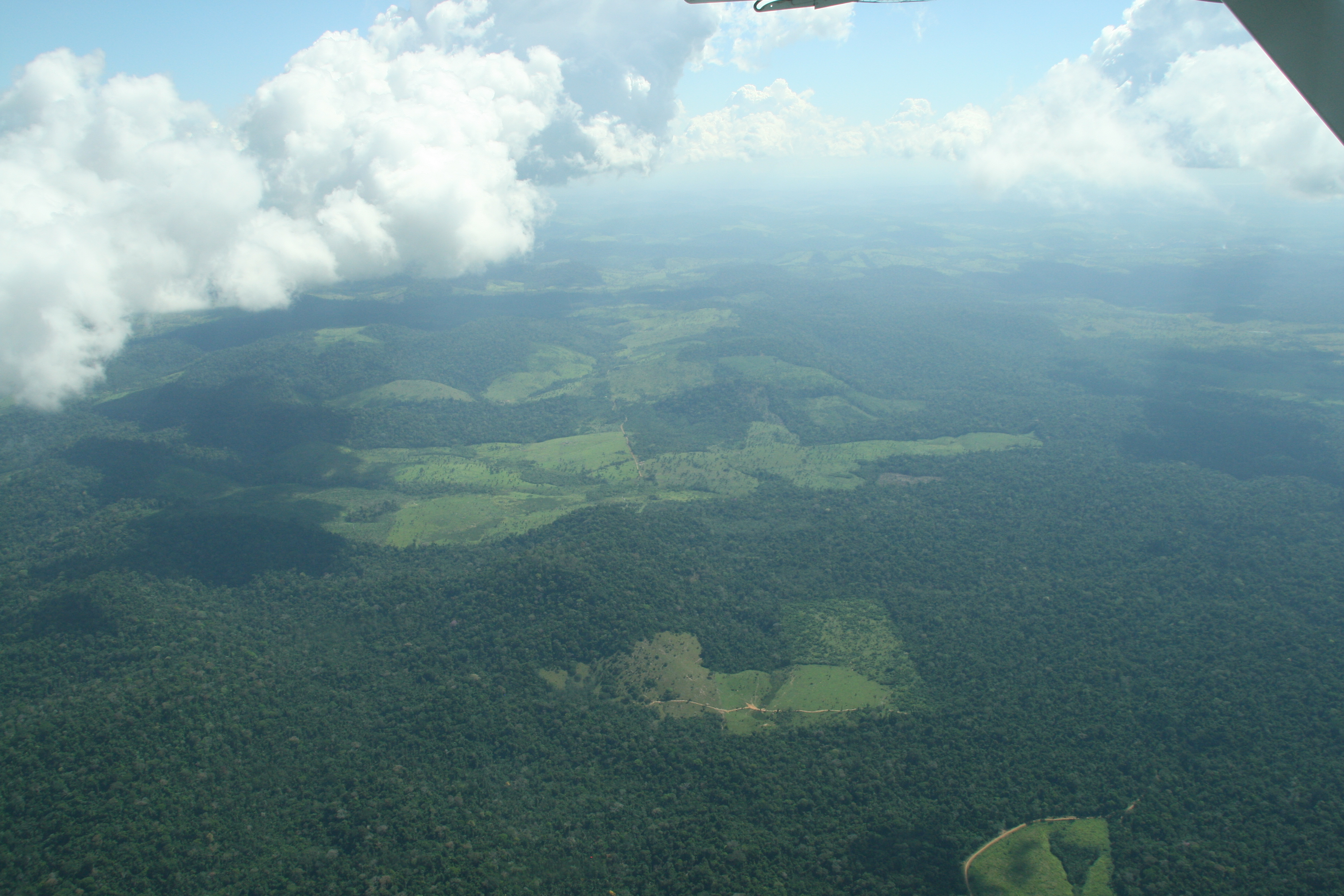
Deforestation processes are widespread across the globe. Remote sensing technologies are often used to map these processes, their spatial patterns, and temporal evolution over large areas. An impressive use case of operational forest monitoring schemes is in Brazil´s Amazon forest. Here, large-area deforestation for cattle ranching and crop cultivation occurs.

Aerial photograph of deforestation in southern Pará, Brazil. Source: Patrick Hostert

The PRODES project, run by the National Institute for Space Research INPE provides information on spatially explicit information of forest loss using visual interpretation of Landsat and CBERS data. Often, however, visual interpretation is not feasible and we desire an automated detection of change processes.

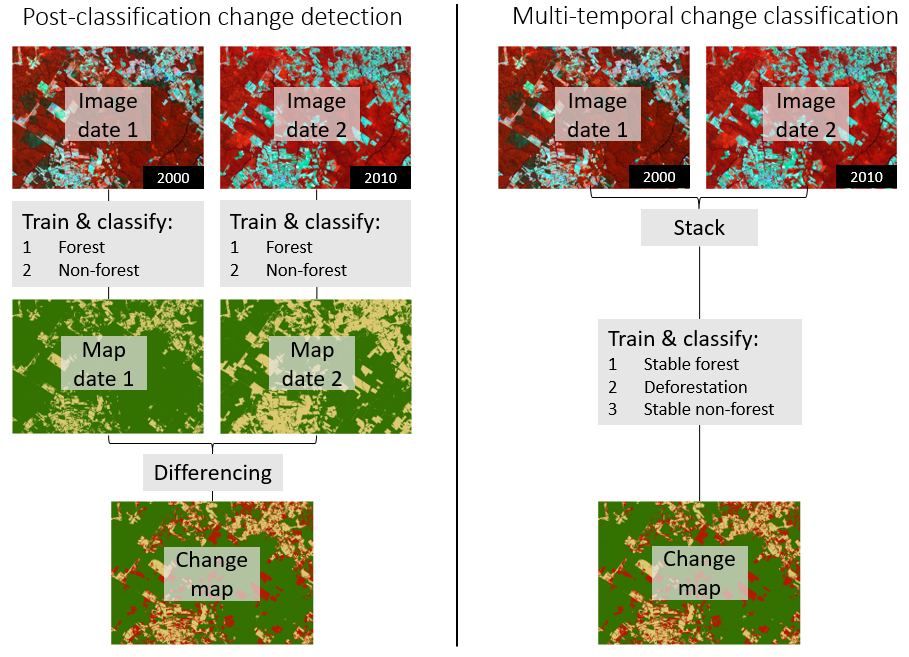
How do we get to the change map? Similar to the production of a land cover map, we can produce maps of land cover or land use change. This inherently incorporates the integration of multiple observation dates. Broadly speaking, change detection can occur in two ways:

Post-classification change detection: This refers to the independent production of land use or land cover maps for each time point of interest. In a next step, differencing techniques are applied to investigate the change between two (or more) maps. While training data collection is relatively straight-forward, error propagation is a core issue for post-classification comparisons. It is therefore advised to assess the map quality of the final change map independently.
Multi-temporal change classification: This refers to the direct classification of a stack of two (or more) images to assess the change classes of interest. Image stacks can be based on reflectance data, vegetation indices, or any other indicators that are comparable over time. Defining good change classes and collecting training data can be challenging. As an example: mapping change between 4 classes A, B, C and D, already requires training data for 16 change trajectories: A-A, A-B, A-C, A-D, B-A, B-B, …, D-C, D-D.

Schematic illustration of change detection methods.

Assignment

After completing the last assignments, you gained a lot of experience in using R & QGIS for data handling and pre-processing, training data collection, classification, and accuracy assessment. In other words: you´re well prepared for performing a change detection study using Landsat data. The goal of this assignment is to map forest cover change in the Southern Brazilian Amazon.

Landsat images of study area for 2000, 2005, and 2010.

We provided the following datasets in our repository:

…sr_data/: Three Landsat 5 surface reflectance stacks (*_crp.tif) at five-year intervals from 2000 to 2010.

LT052260682000061001T1-SC20170927060330 (10 June 2000)
LT052260682005060801T1-SC20170927060440 (08 June 2005)
LT052260682010062201T1-SC20170927060241 (22 June 2010)

…vector/: A shapefile and a *.kmz file for GoogleEarth, which will help you to accurately delineate the Landsat pixel locations and extents for training data collection.

…validation/: A shapefile containing reference data for the accuracy assessment.

…gfc/: A subset of the Global Forest Change dataset by Hansen et al. (2013). We reclassified the data to match the target classes of today´s assignments.

Your task is to create a change map which contains the following classes:

classID	Class
1	Stable forest
2	Deforestation 2001-2005
3	Deforestation 2006-2010
4	Forest gain
5	Stable non-forest

Unlike the previous assignments, you can decide on how the workflow of your map production operates in detail. Use the code and tools from the last sessions and earlier experiences with remote sensing and associated software packages, if applicable. Consider the following steps:

1) Choosing an approach for change detection

Several change detection approaches can be used to map forest cover changes. You can choose a methodological approach for your change detection. We suggest two approaches for supervised classification:

Post-classification comparison: You perform a classification of land cover for each composite dataset. You then use raster algebra in R (or any other tool of your choice) to convert the individual results into a change map.
Integrated multi-temporal change classification: You stack all features into a single file and collect training data for the change classes of interest. You obtain the change map directly from your classification.

2) Screening of input data and training data collection

Visualize the Landsat images in QGIS. Test a true color (RGB), as well as a nIR-swIR1-red false color combination.
Optional: Derive additional features from your data. Do you want to classify based on the spectral bands? What about vegetation indices, principal components, tasseled cap components?
Note that the way in which you collect your training data varies with the approach you choose in the first step.
Collecting training data is time consuming - try to be efficient. Make use of the QGIS Info-Tool to compare spectral profiles of the three images. You can also link QGIS and Google Earth through the Send2GE plugin. For exact pixel boundaries, use the Landsat pixel grid we provided.

3) Model training & classification

Choose a classification algorithm: Feel free to use any classifier. In case you´re interested in differences between classifiers, test more than one.
Parameterize the model. Depending on your choice of classification model, think about how to make an informed decision about the model parameters. Optimize parameters wherever possible, e.g. by using the tuning functions presented in assignment 5.

4) Change map validation & area estimates

We provided reference data for the study area as a shapefile. Use it to perform an accuracy assessment. Why is it challenging to perform an area-adjusted accuracy assessment in this case?
Calculate map-based area estimates for your map and the Global Forest Change data using simple pixel counting. Compare the estimates. What are the major differences?

We collect your main results in this table. Please fill in all required fields, i.e. your name and selected approach (e.g. post-classification comparison), overall accuracy and class accuracies in decimal values (e.g. 0.75), as well as class areas in hectares.

Project choices

For the next session please rank your favorite candidates for the final project work and seminar paper in Moodle. There, you also find the description and overarching guiding/research questions as separate PDF files.