Data quality

Learning goals

Interpret the Landsat Collection 2 quality bands
Produce cloud / cloud shadow masks
Apply the masks on the Landsat L2SP imagery

Background

Landsat data quality

Think about the following question and exchange with your team members:

Which issues affect the data quality of optical satellite images?

How can you find out if a pixel is affected by any of these issues? Luckily, the USGS provides quality bands for the Landsat products.

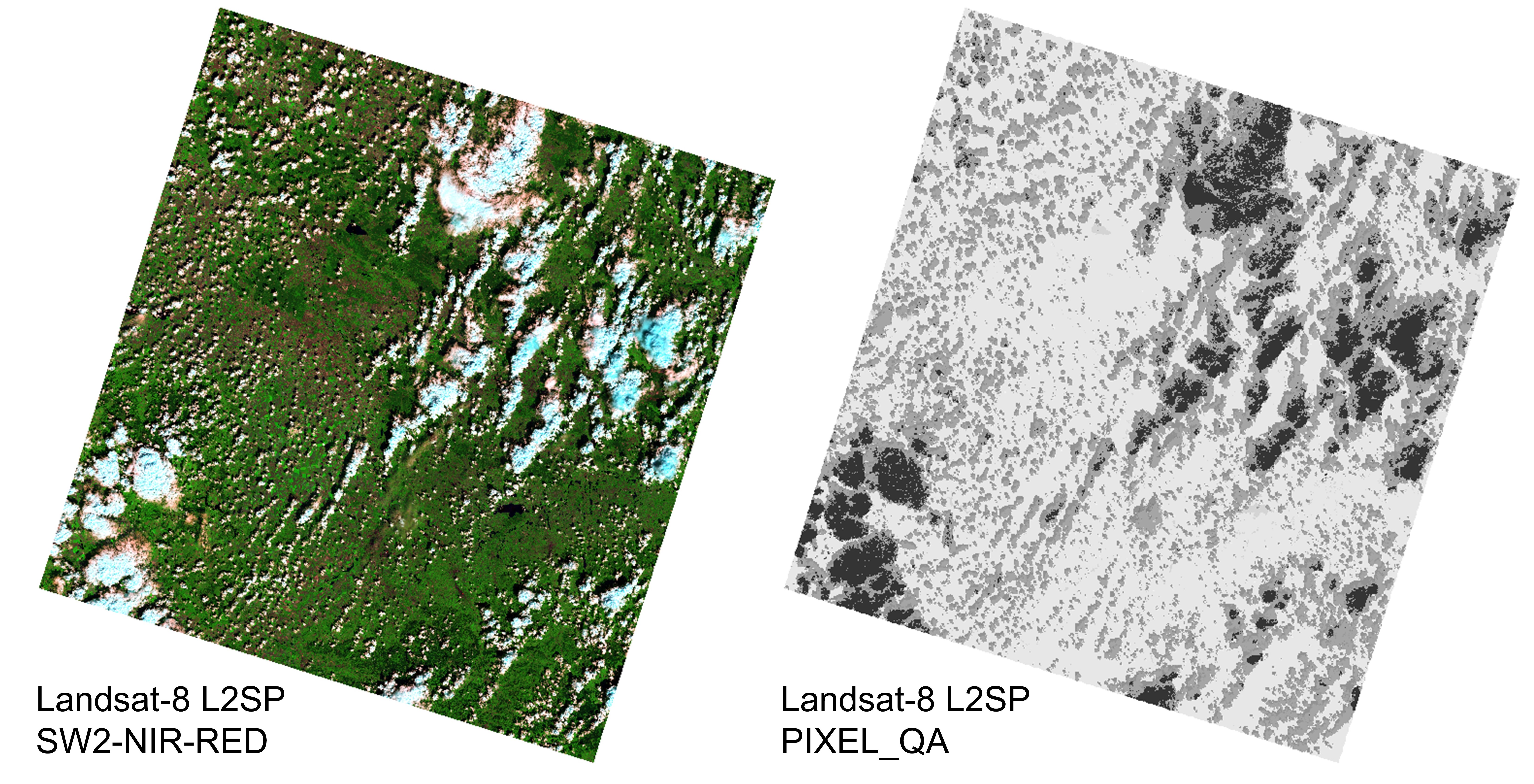
False-color representation of a cloudy Landsat Level 2 image (left) and a grey-scale visualization of the Landsat QA band (right)

If we look up the Landsat QA band website to find out what this band contains, we find the following statement:

“Landsat Collection 2 Level-1 and Level-2 Quality Assessment (QA) bands provide useful information to users wanting to optimize the value of pixels as a first level indicator of certain conditions within Landsat data.”

In the following, you will learn to understand what that means. Please read this section carefully and discuss with your team if necessary.

Landsat QA Bands - Part 1

Before we dive into the realm of the binary system, let us have a look at what the Landsat Quality Assessment Bands, particularly the QA_PIXEL band, provide us with. If we zoom into the QA_PIXEL image depicted above, we are able to delineate individual patterns of pixels and their respective values:

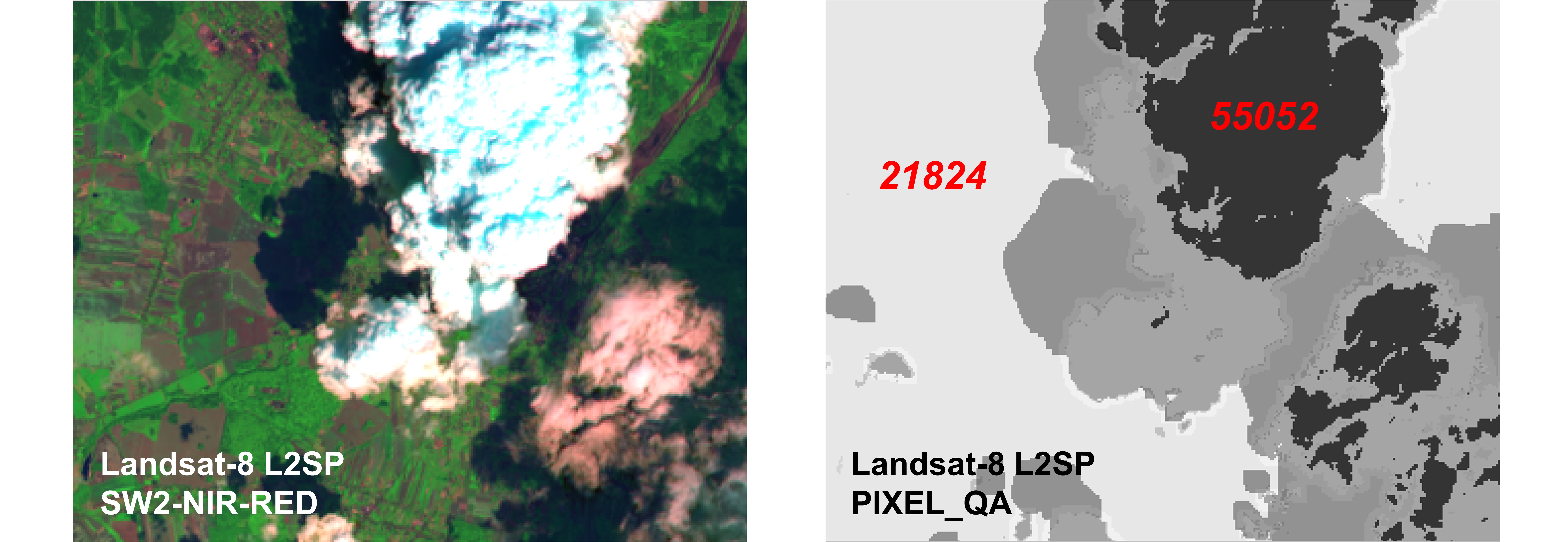
Zoom-in on false-colour image (left) and associated QA_PIXEL image-file (LC08_L2SP_189025_20140716_20200911_02_T1_QA_PIXEL) (right.)

We can identify, for example, that the clear-sky pixels have an assigned integer value of 21824 while the pixels in the center of the cloud have an assigned integer value of 55052. If we had a look at all identifiable pixels, we could observe that other regions, including the clouds and cloud shadows, have yet again unique integer values.

The QA_PIXEL band thus provides us with information associated with unique states or qualities for each pixels. If we aim at masking out clouds and other factors we treat as noise, we can make use of this information. But how?

We will see that the integer values are - similar to DNs - just an elegant way of storing a multitude of information in single integer values. For the information to be interpreted by us, however, we need to decode the values into their binary representation.

The binary system

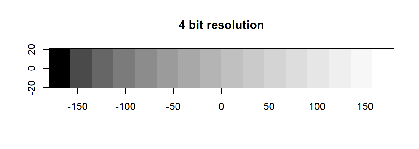
Recall from just now that we quantized the radiometric resolution of a sensor in bits:

Do you know the binary numeral system (0 / FALSE or 1 / TRUE)?

The binary system represents numbers through sequences of bits (binary digits). Each bit has a position and a state. The positions are numbered from 0 to the total number of bits, usually read from right to left. The state of an individual bit can either be 0 (FALSE) or 1 (TRUE). From an electric circuits perspective, electricity is either off (0) or on (1). Consider the meaning of 0 as “FALSE” or “NO”, 1 equals “TRUE” or “YES”. These building blocks are essentially the two states on which all software is ultimately built upon.

We can represent all sort of ideas in binary, including - of course - numbers and letters. A number in binary is a number expressed in the base-2 numeral system (0 and 1, instead of 0, 1, 2, 3, 4, 5, 6, 7, 8, 9 in decimal). Just like in the decimal system, however, if we want to represent quantities beyond the amount of unique digits available (0-1 for binary, 0-9 for decimal), we ‘flip over’ to an additional position, re-starting the count on the previous position (in decimal this would be 1, 2, ..., 9, -> flip -> 10, 11, ..., 99 -> flip -> 100, 101, ..., 999 -> flip -> 1000, ...). Hence if we run out of symbols, we add a new position.

Let us image we start counting from 0 to 10 in binary:

0 -> 0
1 -> 1 - now we already run out of symbols, so for the next count we add a position
2 -> 10
3 -> 11 - again, we add a position for the next count
4 -> 100
5 -> 101
6 -> 110
7 -> 111 - again, we add a position for the next count
8 -> 1000
…

Since a binary system operates in base 2, each bit position is assigned a unique value defined by \(2^{n}\), where n is the bit position starting at 0. So for bit position 0, we have a value of \(2^{0} = 1\), for bit position 1 we have a value of \(2^{1} = 2\), for bit position 2 we have a value of \(2^{2} = 4\), and so on. When extracting values from the entire bit sequence, we can simply add together all bit positions which have a state of 1 (TRUE). The visualization of the described looks as follows:

The binary number system. The bit position n (purple) and resulting value from \(2^{n}\) (blue) and bit state (orange) Source: Wikipedia

In the example above, five bit positions are given, hence the quantization is 5-bit. We can see that different combinations of states and positions enable us to represent any integer number, limited only by the number of bits in the sequence.

The more bits in a sequence we have, the higher the numbers we can generate. With 5 bits, we can represent the numbers 0–31 (i.e., 32 unique values), with 16 bits, we can represent the numbers 0 - 65,535 (i.e., 65,536 unique values).

Such a system can be used to assign digital numbers or reflectance values to a pixel in a raster dataset. Alternatively, bit positions can be assigned any meaning a user likes. For example, letters can be assigned based on their position in the alphabet, as seen with the encoded message on the Perseverance rover’s parachute during its Mars landing.

Binary was used to encode NASA JPL’s motto and coordinates on the Perserverance lander’s parachute

In the next section, we will see how bit positions in the Landsat Quality Assessment (QA_PIXEL) band can be used to determine a pixel’s quality based on a number of different criteria.

Landsat QA Bands - Part 2

Back to our QA_PIXEL bands: The Landsat QA band is coded in 16-bit, hence a pixel lies within the range between 0-65,535. What we are interested in, is the binary representation of a given integer value. For example, in the example above we observed pixels in the center of the cloud to exhibit a value of 55052. Now we can convert this into its binary form.

R offers a good way of dealing with bit-packed information. The intToBits() function converts integer numbers into sequences of bits, whereas 32 double-digit bits are returned by default. We convert the double digits to single digits using as.numeric() and revert the bitstring rev() since we usually read them from right to left

# Convert the double-digit into single-digit bits
rev(as.numeric(intToBits(55052)))

##  [1] 0 0 0 0 0 0 0 0 0 0 0 0 0 0 0 0 1 1 0 1 0 1 1 1 0 0 0 0 1 1 0 0

We´re looking at 16 bit data, so let´s deprecate the unused bits

# We´re looking at 16 bit data, so let´s deprecate the unused bits
rev(as.numeric(intToBits(55052)[1:16]))

##  [1] 1 1 0 1 0 1 1 1 0 0 0 0 1 1 0 0

The 16-bit string representation of this number (1 1 0 1 0 1 1 1 0 0 0 0 1 1 0 0) can now be compared to the unique meanings of the bit positions, defined by the USGS as follows:

Landsat Collection 2 Level-2 QA_PIXEL band bit designation

We have the bit positions in the left column (Bit), the meaning of the psoition in the center (Flag Description) and the meaning of the state on the right (Values). Accordingly, each bit has a specific meaning in terms of data quality. For example, bit position 4 (i.e., 5th entry since we start at 0) means “cloud shadow”. If bit 4 has the state 1 (“YES” | “TRUE”), there was a cloud shadow detected in that pixel. If it has the state 0 (“NO” | “FALSE”), there were no cloud shadows detected in that pixel.

In the Landsat QA band, there are additionally single (bit positions 0 to 7) and double bits (bit positions 8 to 15). Single bits inform about one condition in a binary manner:

Single bits (bit 0, 1, and 4):

0 = “No” = The condition does not exist.
1 = “Yes” = The condition does exist.

Double bits can represent conditions in more detail. In the case of the QA_PIXEL band, double bits represent levels of confidence that a condition exists:

00 = “Not Determined” = Algorithm did not test for the condition.
01 = “Low” = Algorithm has low confidence that this condition exists (probability of 0-33%).
10 = “Medium” = Algorithm has medium confidence that this condition exists (probability of 34-66%).
11 = “High” = Algorithm has high confidence that this condition exists (probability of 67-100%).

In addition to the meaning assigned to each bit position, the entire bit sequence of the QA band can be read as an integer value just like any of the reflectance bands. For example, take a pixel where bit 4 has the state 1 and all other bits have the state 0. This indicates a cloud shadow pixel, but the resulting integer value of the entire bit sequence (0000000000010000) will be \(2^{4} = 16\). If the confidence in shadow detection of the algorithm is “medium/reserved”, bit positions 10-11 are assigned 10, which changes the entire 16-bit string to 0000100000010000. Thus the integer value of the new bit sequence will be \(2^{4} + 2^{11} = 2064\). Following this logic, different combinations of true/false conditions will result in different integer values.

Please note that bit designations vary between sensors and data products. Collection 2 data differs from Collection 1, BOA products (L2SP) might differ from TOA (L1TP). For Landsat data, carefully check the USGS website prior to your quality masking.

21824

55052

Investigating the QA band

Let´s have a look at the Landsat Collection 2 Quality Band (QA_PIXEL) of the surface reflectance product (L2SP) (LC08_L2SP_189025_20140716_20200911_02_T1)

freq()

As you can see, the band contains many integer values. By decoding the integer values into 16 bit binary strings, we can read the quality information for each pixel. Use the intToBits() function to decode the three most frequent BQA values. As shown above, intToBits() returns 32 bits by default. Make sure you only look at bits 1 to 16. Also, keep in mind the right-to-left order when comparing the decoded bits with the table. You might want to use rev() to invert the order of the outputs by intToBits().

Decipher the meaning of the three most frequent values.

Note your findings as a comment in the script:

# What do the most frequent values mean? Decode each integer value into bits and 
# describe their meaning here: 

# Most frequent value + meaning as comment
# Second most frequent value + meaning as comment
# Third most frequent value + meaning as comment

2) Creating a cloud mask

By converting integer values into binary bits, we can extract specific attributes from the BQA by applying user-defined logical statements. Let´s to this in a systematic manner by defining a function, which yields TRUE where bit position 0 equals 1, hence designated fill pixels (empty areas around the tilted rectangle containing actual observations):

# Define function to find fill values from Landsat QA_PIXEL
fill_pixels <- function(x){
  return(intToBits(x)[1] == T)
}

Note: R (e.g. in contrast many other languages) starts indexing at [1] not [0]. Thus bit position 0 is located at position [1] in the numeric vector. The function has one input, which is expected to be an integer which gets converted into a vector containing the binary representation of the integer.

Use indexing and Boolean expressions to define new functions which return TRUE for:

high confidence clouds OR high confidence cloud shadows OR fill values
high AND medium confidence clouds OR high AND medium confidence cloud shadows OR fill values

Then, create the two mask images using the above functions on your QA_PIXEL raster object.

Overview of terra methods
In general, you can apply functions (including user-defined functions) on rast objects on each pixel (app) or each layer (band) separately (sapp). In our case, the indexing of the intToBits() output within the function currently leads to a wrong behaviour within the app function, therefore we circumvent this by working directly on the array of the rast object:

# extract values from rast-object into array
val_qa <- values(img_qa)  # img_qa is the reprojected QA rast-object
val_mask <- sapply(val_qa, fill_pixels)  # apply function to each element and return vector 
# terra::setValues takes a blueprint raster (img_qa) and fills the provided values (val_mask) 
# into a new raster (img_mask):
img_mask <- setValues(img_qa, val_mask)

Plot the mask and check if clouds, cloud shadows, and fill values are labeled as 1 and clear observations as 0.

Create a binary mask from each function.
Discuss and decide on the appropriate data type for binary masks and write them to disk.

Open both masks in QGIS, together with an RGB representation of the image.

Which mask is more reliable in your opinion?

3) Masking images

Apply the mask onto the BOA-stack and write the masked image to disc.

Load the BOA data as a stack (VIS, nIR, swIR) and use the mask() function to mask clouds, cloud shadows and fill values from the image. Use the mask which you found to be more accurate. Make sure to specify the maskvalue argument accordingly. Write the masked BOA stack to disk in the GTiff format.

Reading materials

For the next session, please read sub-chapter 7.1 of chapter 7 in Chuvieco (2020) (i.e. pages 235-263):

Chuvieco (2020): Fundamentals of Satellite Remote Sensing : An Environmental Approach, Chapter 7

Sub-chapter 7.1 (p. 235-263) focuses on the estimation of variables using indices and transformations and their relation to biophysical surface properties. Our focus lies on the theory and application of the presented concepts, you do not have to dive deeply into all mathematical notations (although this can help towards achieving a better and more comprehensive understanding of the topics).

While reading focus on the following questions:

What are key reasons for performing Principle Component Analysis (PCA), deriving Tasseled Cap (TC) components or calculating Vegetation Indices (VIs)?
What are benefits of using TC over PCA - and vice versa?