Higher level image features - I

Best-Available-Pixel (BAP) compositing

Learning goals

Understand the fundamentals of best-available-pixel (BAP) image compositing
Parameterize a BAP compositing function and create your own BAPs

Background higher level image features

The availability of Landsat images varies by region. Even in areas where observation density is high, such as North America, coverage can be reduced by clouds and quality of observations can be impacted by haze or sensor saturation.

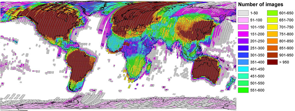
Global availability of Landsat images. Source: Wulder et al. 2016; https://doi.org/10.1016/j.rse.2015.11.032

Using best-available-pixel (BAP) compositing or generating spectral-temporal-metrics (STMs), we can integrate multiple observations (e.g., from multiple Landsat images) into gap-free higher level image features. This not only enables large area mapping - as described in Griffith et al. (2013) - but also collapses the (dense) time series into fewer dimensions (less bands), reducing computational costs while preserving or even amplifying the variance in the data.

Best-Available-Pixel compositing

One of the first global Landsat composites was produced using the WELD compositing approach (Roy et al. 2011, https://doi.org/10.1016/j.rse.2009.08.011).

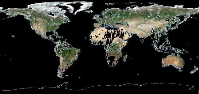
Monthly global WELD surface reflectance composite for June 2009. Source: https://worldview.earthdata.nasa.gov/

Pixel-based compositing allows us to create cloud-free, radiometrically and phenologically consistent image composites that are contiguous over large areas. A set of parameters is used to determine the observations best suited for analysis. These parameters can, e.g., include the distance to clouds in the image, or the temporal proximity to a target day of the year (DOY). Defining scoring functions allows for a flexible parametrization according to user’s needs and study area characteristics. Different parameters can also be weighted according to their relevance for a given application.

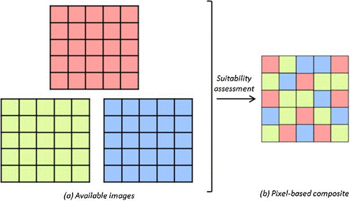
Creating one best-pixel composite from three images.

BAP compositing in 7 steps

1) Input data

Generally, a multitude of approaches to image compositing exist. Here we take a closer look at the specific method by Griffith et al. (2013). First, let us define the needed input data to create BAP composites:

Cloud-masked (or accompanied by cloud masks) multitemporal image acquisitions (preferable surface reflectance for radiometric consistency)
Pixel-wise cloud distance layers of the multitemporal image acquisitions

For example, the figure below depicts a subset of the multitemporal imagery showing five distinct cloud-masked image acquisitions and the associated cloud distance layers.

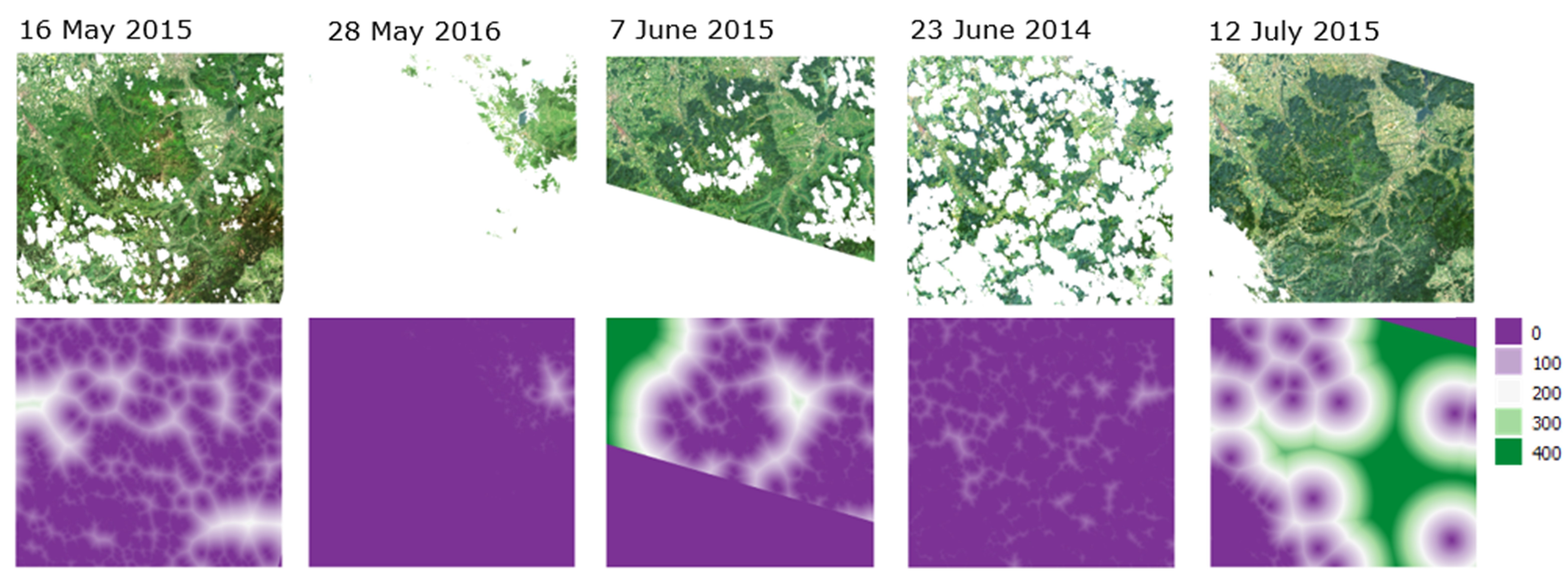
Five images to be used for best-pixel compositing and their DOY and year offsets

2) Determine main compositing parameters

We use compositing parameters to determine the ‘best’ pixels for our composite. The main compositing parameters include the target DOY (target_doy), target year (target_doy), and the distance to clouds (cloud_dist) of a given pixel (e.g. in meters). As an example, our goal will be a peak-of-season (mid-summer) composite with a focus on seasonal consistency. Thereby, we define the three target compositing parameters as:

target_doy = 195
target_year = 2015
cloud_dist is a raster layer calculated based on our cloud mask (see below)

Next we can adjust each of the suitability functions by defining the preferred seasonal and annual windows as well as the minimum and maximum distance to clouds.

3) Parameterize scoring functions

We will use a Gaussian function to determine the DOY suitability of an observation. In the plot for the DOY function below (left), we’re choosing a parameterization that favors observations closer to the target DOY and assign a suitability score of 0 for observations >50 days from the target date, thus:

max_doy_offset = 50

For example, a May 16 2015 observation is 30 days from the target DOY and receives a suitability score of 0.19.

A linear function determines the suitability score for the year of observation (plot below, right). Again, observations close to the target year are assigned high values, while observations acquired five or more years from the target year are considered unsuitable, thus:

max_year_offset = 5

The resulting suitability score for the May 15 2015 observation is 1.

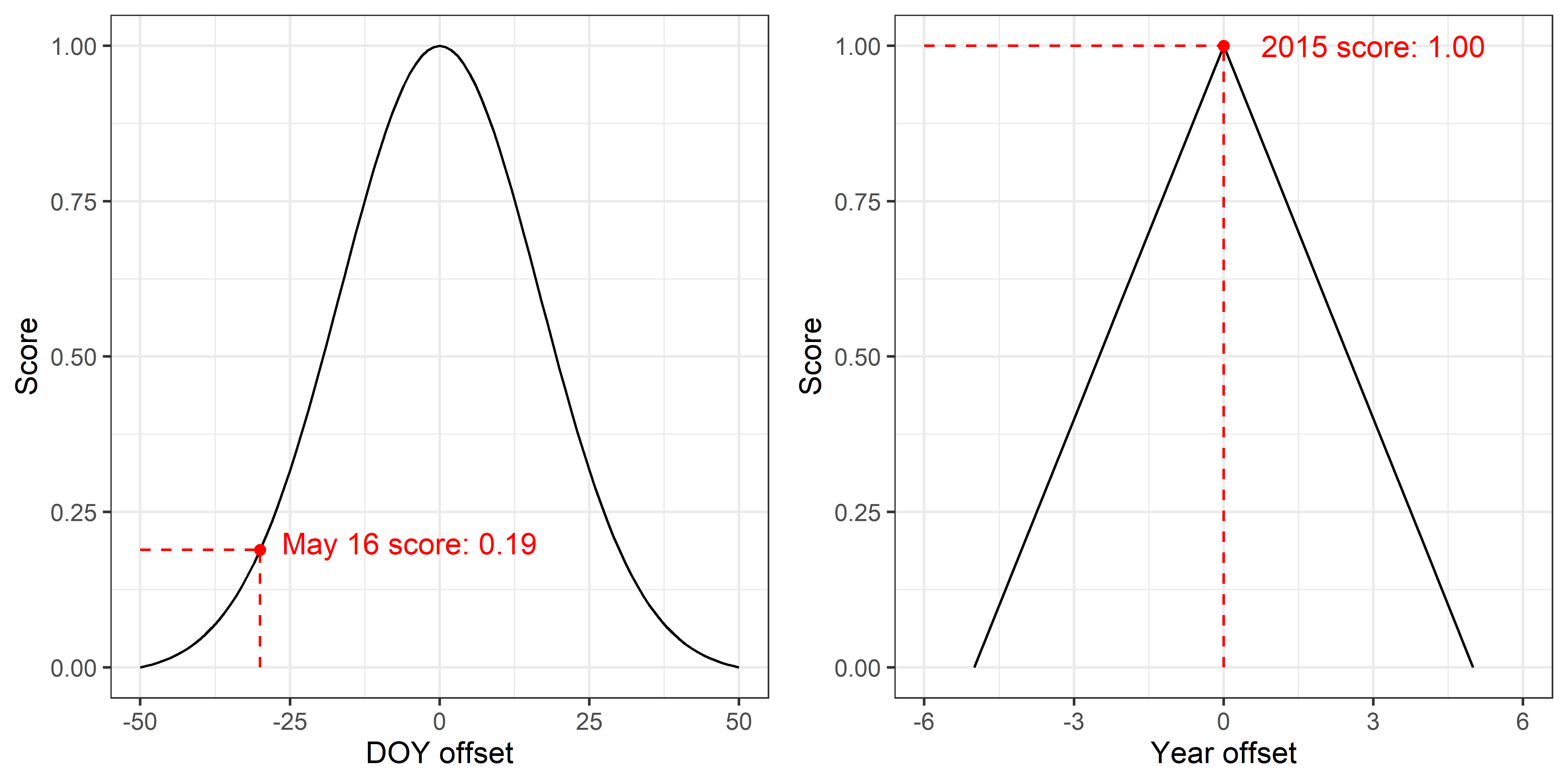
Scoring functions for the DOY and year suitability score

Last, to minimize the likelihood of pixels being affected by clouds, we favor observations further away from clouds. The linear cloud distance scoring function below assigns a suitability score of 1 as soon as the distance to the next cloud is equal or greater than 100 pixels. Pixels with <10 pixels distance from clouds are treated as unsuitable with a score of 0. Accordingly:

min_cloud_dist = 10 (here we used pixels, the implementation down below for the assignment uses the coordinate systems unit, e.g. meters)
max_cloud_dist = 100

For example, an observation that has a distance of 60 pixels (approximately 1800m) to the next cloud receives a cloud distance suitability score of 0.56.

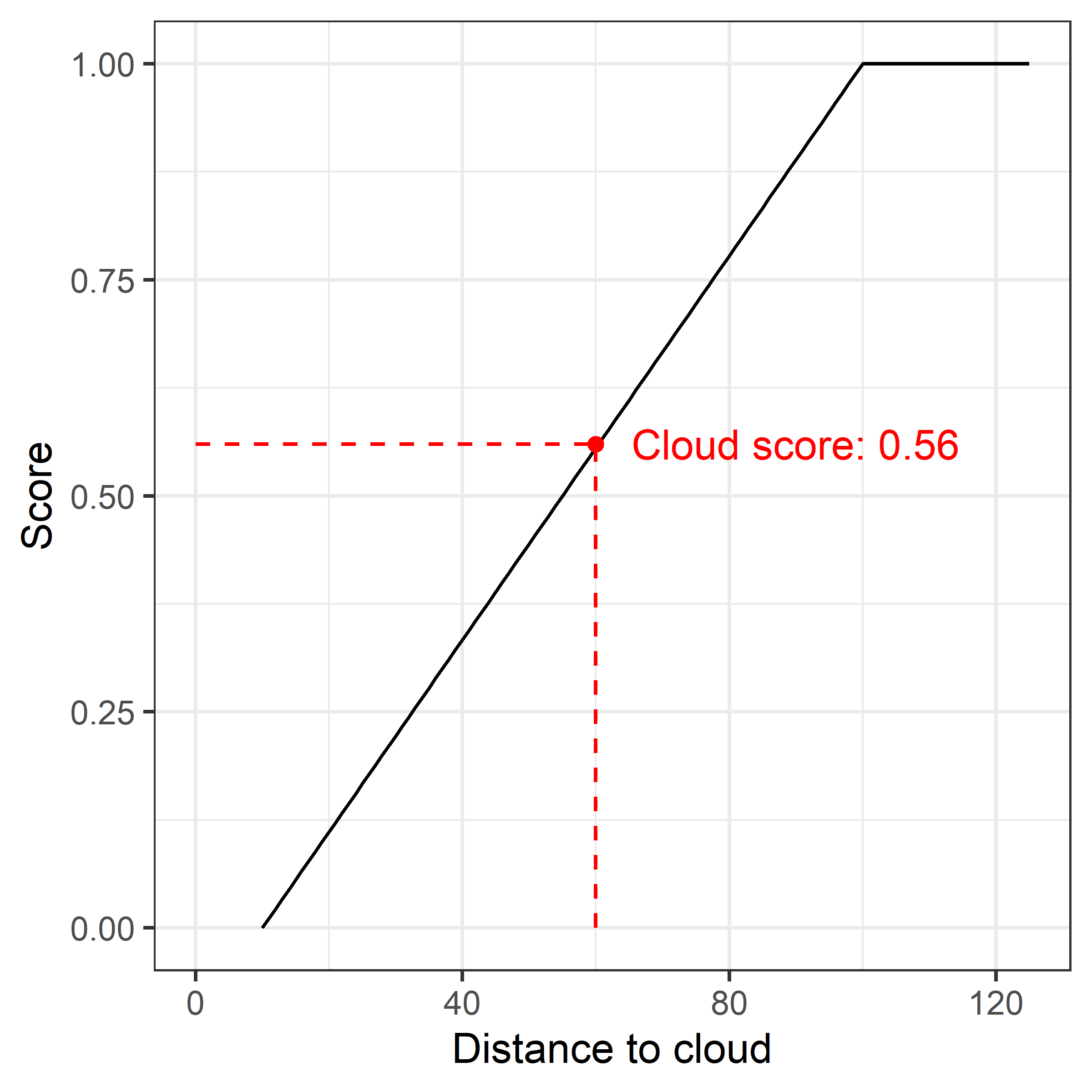
Linear function for the cloud suitability score

4) Define parameter weights

Next, we can define the importance of the different parameters according to our needs by defining weights for each of the suitability scores. For instance, by prioritizing the DOY score over the year score (i.e., seasonal consistency rather than annual consistency):

w_doy = 0.5
w_year = 0.2
w_cloud_dist = 0.3

5) Calculate a score for each pixel in each image.

Now we can retrieve the weighted sum of suitability score for each pixel in each image:

score = score_doy * w_doy + score_year * w_year + score_cloud * w_cloud_dist

Using the values from the example above yields:

score = 0.19 * 0.50 + 1.00 * 0.20 + 0.56 * 0.30 = 0.463

6) Use the best observation (i.e. the highest score) for each pixel to create the final composite.

7) Evaluate the results by checking for seasonal/annual consistency and cloud distance (and re-iterate).

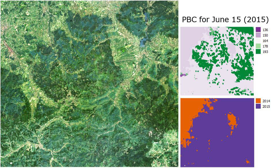
Final Landsat composite and Pixel Based Composite (PBC) information

Assignment

The goal of this week’s assignment is to combine several images into best-pixel composites using a parametric compositing function. We use the data from the previous session found here. Let’s revisit the content of the folders needed fot todays session:

Preprocessed Landsat-7 and Landsat-8 band-wise (blue, green, …) surface reflectance time series from 2014 to 2016 ("/imagery/time-series")
Cloud distance (in m) raster stack complementing the surface reflectance time series ("/imagery/bap/2014-2016_001-365_HL_TSA_LNDLG_CDS_TSS.tif")
Valid/non-cloud pixel mask complementing the surface reflectance time series ("/imagery/bap/2014-2016_001-365_HL_TSA_LNDLG_VLD_TSS.tif") (this is important since we have fill values and include Landsat-7 data with SLC-off data gaps which we need to mask during the BAP calculation)

Today we will be working with pre-defined scripts. We provide both, (1) a script containing the compositing function and (2) a main script which sources and executes the compositing function. Outsourcing functions - especially complex ones - improves the readability of scripts and allows for using the same functions in different files. Check the help for source() if you are not familiar with sourcing R code in your script. You can find both scripts below. Please copy them into two separate R files and save them into your working directory.

Click here to view the parametric compositing function

# =============================================================================
# GCG - EARTH OBSERVATION
# BEST AVAILABLE PIXEL (BAP) COMPOSITING
# based on Griffith et al. 2013
# L. Nill, 2022; update 2023
# =============================================================================

# =============================================================================
# load required packages
library(terra)

# =============================================================================
# scoring function
bap_score <- function(doy, year, cloud_dist, target_doy, target_year, 
                      w_doy=0.5, w_year=0.2, w_cloud_dist=0.3,
                      max_doy_offset=30, max_year_offset=1,
                      min_cloud_dist=0, max_cloud_dist=1000, 
                      valid_pixels=NULL){
  "Function to calculate BAP score based on provided DOY, year and cloud 
  distance information. Supplied objects must exhibit the same length to be
  braodcasted together.
  
  doy:            (numeric) Vector containing DOYs. Must be of same length as 
                  cloud_dist.
  year:           (numeric) Vector containing Years. Must be of same length as 
                  cloud_dist.
  cloud_dist:     (raster) Raster object representing distance to clouds (unit 
                  must match min_cloud_dist and max_cloud_dist)
  target_doy:     (int) Target day-of-year (mean of Gaussian PDF)
  target_year:    (int) Target year (peak - score = 1 - of piecewise linear)
  w_doy:          (float) Weight associated with the DOY score 
  w_year:         (float) Weight associated with the year score
  w_cloud_dist:   (float) Weight associated with the cloud distance score
  max_doy_offset: (int) Maximum offset from 'target_doy' at which score = 0 
  max_year_offset:(int) Maximum offset from 'target_year' at which score = 0
  min_cloud_dist: (int) Minimum distance (unit as in 'cloud_dist') at which
                        score = 0
  max_cloud_dist: (int) Maximum (and greater than) distance (unit as in 
                        'cloud_dist') at which score = 1
  valid_pixels:   (rast, optional) Optional mask layer. 1 = valid, 0 = invalid
  
  returns:        (list) Raster (stack) containing pixel-wise index of maximum 
                  score [[1]], maximum score [[2]], doy [[3]] and year [[4]] of 
                  maximum score.
  "
  
  # assert if weights sum up to 1
  if (sum(w_doy, w_year, w_cloud_dist) != 1){
    stop("Error: Specified weights NEQ 1")
  }
  
  # assert if doy, year, cloud_dist are of same length
  zdim <- dim(cloud_dist)[3]
  if (length(unique(c(zdim, length(year), length(doy)))) != 1){
    stop("Error: Inputs doy, year, cloud_dist of different length")
  }
    
  # 1) DOY score (Gaussian kernel)
  print("1/5 Calculating DOY score.")
  score_doy <- exp(-0.5 * ((doy - target_doy) / (max_doy_offset/3))^2)

  # 2) Year score
  print("2/5 Calculating YEAR score.")
  score_year <- 1-(abs(target_year - year) / (max_year_offset+0.1))
  
  # plot year and doy scoring
  par(mfrow=c(2,1))
  plot(seq(0,365,1), exp(-0.5*((seq(0,365,1)-target_doy)/(max_doy_offset/3))^2),
       type = "l", xlab="Day of Year", ylab="Score")
  points(doy, score_doy, col=factor(year), lwd=1)
  legend("topleft",
         legend = levels(factor(year)),
         pch = 1,
         col = factor(levels(factor(year))))
  plot(seq(min(year)-1,max(year)+1,1), 
       1-(abs(target_year-seq(min(year)-1,max(year)+1,1))/(max_year_offset+0.1)),
       type = "l", xlab="Day of Year", ylab="Score")
  points(year, score_year, col="red")

  # 3) Cloud score
  print("3/5 Calculating cloud_dist score.")
  cloud_dist <- terra::classify(cloud_dist, rcl=c(0, min_cloud_dist, NA), right=NA, 
                      datatype='INT2S')
  cloud_dist <- terra::classify(cloud_dist, rcl=c(max_cloud_dist, Inf, max_cloud_dist), right=NA, 
                      datatype='INT2S')
  score_cloud <- (cloud_dist - min_cloud_dist) / (max_cloud_dist - min_cloud_dist)
  
  # net score
  print("4/5 Calculating NET score.")
  score <- score_doy*w_doy + score_year*w_year + score_cloud*w_cloud_dist
  if (!is.null(valid_pixels)){
    score <- score * valid_pixels
  }
  
  # get index of maximum score and associated scores
  print("5/5 Calculating index of MAX score.")
  idx_max <- which.max(score)
  score_max <- max(score, na.rm=T)
  
  # look-up for year and doy raster
  lu_doy <- cbind(1:zdim, doy)
  lu_year <- cbind(1:zdim, year)
  doy_max <- terra::classify(idx_max, rcl=lu_doy, right=NA, datatype='INT2S')
  year_max <- terra::classify(idx_max, rcl=lu_year, right=NA, datatype='INT2S')
  
  out_stack <- terra::rast(list(idx_max, score_max, doy_max, year_max))
  names(out_stack) <- c("idx", "score", "doy", "year")
  plot(out_stack)
  
  print("Done.")
  return(out_stack)
}

# =============================================================================
# function to create composites from imagery based on suitability/score layer

create_bap <- function(img_raster, idx_raster){
  "Function to create BAP composite from raster stack using index raster.
  
  img_raster:   (raster) Input (3D) image data for compositing.
  idx_raster:   (raster) Input (2D) index raster containing pixel-wise index
                along z-dimension of img_raster.
  
  returns:      (raster) Best-available-pixel composite (2D) image
  
  "
  # get unique selected scenes only
  idx_unique <- unique(idx_raster, na.rm=TRUE)
  img_raster <- img_raster[[idx_unique]]
  # reset index (because of sub-selection)
  idx_raster <- terra::classify(idx_raster, 
                           rcl=cbind(idx_unique, 1:dim(img_raster)[3]))
  # read data into matrices
  img_matrix <- as.matrix(img_raster)
  idx_matrix <- as.vector(idx_raster)
  bap <- img_matrix[cbind(seq_len(nrow(img_matrix)), idx_matrix)]  # index
  bap <- terra::rast(nrows=nrow(img_raster), 
                ncols=ncol(img_raster), 
                crs=crs(img_raster), 
                vals=bap,
                ext=ext(img_raster))
  return(bap)
}

# EOF

Click here to see the script calling the compositing function

# =============================================================================
# GCG - EARTH OBSERVATION
# SESSION 4: Higher level image features
# Name, Name, ...
# =============================================================================

# =============================================================================
# load required packages
l_packages <- c("terra", "lubridate")
for (p in l_packages){
  if(! p %in% installed.packages()){
    install.packages(p, dependencies = TRUE)
  }
  library(p, character.only = T)
}

# =============================================================================
# Part I - Best-Available-Pixel compositing
# =============================================================================

dir_main <- '...\session_03-06'
setwd(dir_main)

# =============================================================================
# 1) Prepare input

# create list of desired image band files
l_bands <- c("BLU", "GRN", "RED", "NIR", "SW1", "SW2", "NDV", "EVI", "TCG", 
             "TCB", "TCW")
l_files <- sapply(l_bands, function(x){
  paste0("imagery/time-series/2014-2016_001-365_HL_TSA_LNDLG_", x, "_TSS.tif")
})
print(l_files)

# read raster stacks
l_stacks <- lapply(l_files, terra::rast)

# retrieve necessary variables for compositing (DOYs and year vectors)
bandnames <- names(l_stacks$BLU)
datestring <- lapply(bandnames, function(x) as.Date(substr(x, 1, 8), "%Y%m%d"))
doys <- as.numeric(lapply(datestring, yday))
years <- as.numeric(lapply(datestring, year))

# read cloud distance and valid pixels (masks) stacks
cdists <- terra::rast('imagery/bap/2014-2016_001-365_HL_TSA_LNDLG_CDS_TSS.tif')
vld <- terra::rast('imagery/bap/2014-2016_001-365_HL_TSA_LNDLG_VLD_TSS.tif')


# =============================================================================
# 2) Parameterization

# path to the bap_compositing-function including .R suffix
source('...')

# Composite 1
# parameters
target_year <- 2015
target_doy <- 0

w_year <- 0.0
w_doy <- 0.0
w_cdist <- 0.0

max_doff <- 0
max_yoff <- 2

min_cdist <- 0
max_cdist <- 0

# call bap_score-function for 1st composite
bapscore1 <- bap_score(doy=doys, year=years, cloud_dist=cdists, 
                       target_doy=target_doy, target_year=target_year, 
                       w_doy=w_doy, w_year=w_year, w_cloud_dist=w_cdist, 
                       max_doy_offset=max_doff, max_year_offset=max_yoff, 
                       min_cloud_dist=min_cdist, max_cloud_dist=max_cdist,
                       valid_pixels=vld)

# create composites for each band from index object
l_composites <- lapply(l_stacks, create_bap, idx_raster=bapscore1$idx)

# create stack of composite rasters + DOY and YEAR info and write to disc
comp <- terra::rast(c(l_composites, bapscore1$doy, bapscore1$year))
print(comp)

outname <- paste0('imagery/bap/LNDLG_BAP_Y', toString(target_year), '-', 
                  toString(max_yoff), '_DOY', toString(target_doy), '-', 
                  toString(max_doff), '.tif')
writeRaster(comp, outname, datatype = 'INT2S', overwrite=T)

# Composite 2
# ...


# =============================================================================
# Part II - Spectral-Temporal-Metrics
# =============================================================================
# ...

1) Parameterization: defining target dates and parameters

Define the parameterization for two composites and briefly comment on your decisions.

The function above allows you to produce BAP composites. It requires the input of the variables mentioned above and below the function definition:

"""
doy:            (numeric) Vector containing DOYs. Must be of same length as 
                cloud_dist.
year:           (numeric) Vector containing Years. Must be of same length as 
                cloud_dist.
cloud_dist:     (rast) Raster object representing distance to clouds (unit 
                must match min_cloud_dist and max_cloud_dist)
target_doy:     (int) Target day-of-year (mean of Gaussian PDF)
target_year:    (int) Target year (peak - score = 1 - of piecewise linear)
w_doy:          (float) Weight associated with the DOY score 
w_year:         (float) Weight associated with the year score
w_cloud_dist:   (float) Weight associated with the cloud distance score
max_doy_offset: (int) Maximum offset from 'target_doy' at which score = 0 
max_year_offset:(int) Maximum offset from 'target_year' at which score = 0
min_cloud_dist: (int) Minimum distance (unit as in 'cloud_dist') at which
                      score = 0
max_cloud_dist: (int) Maximum (and greater than) distance (unit as in 
                      'cloud_dist') at which score = 1
valid_pixels:   (rast, optional) Optional mask layer. 1 = valid, 0 = invalid
"""

In the provided script, the data is already prepared for direct input and the associated DOY and year vectors are extracted from the bandnames. Relying on last week´s insights during training data collection, define two target days of the year (DOY) for two different composites to capture contrasting phenological stages of the different forest types. This includes making a decision concerning the compositing parameters explained in the background section.

2) Running and exploring the parametric compositing function

Create your first composite based on your parameterization and write the result to disk (as provided in code above).

While the code is executing, have a closer look at the function:

Comprehend the compositing function by defining the variables and the code within the function line-by-line.
Mark parts you might not comprehend. We can clarify them as group.

Open the .R script containing the function and take time to read through it in groups. Define the necessary parameters and objects (see above) and run the script line by line. Investigate the outcomes of each line and discuss questions in your group. Seek the help pages of functions you do not yet know.

4) Visual inspection and evaluation of results

Visually inspect the quality of your compositing results in QGIS. Look at the bands containing the DOY and year flags (last two bands).

What worked out well. What did not? How could the quality of the composites potentially be improved?
Re-iterate with different parameters if you evaluate the composites might not be suited for classifying different forest types.