Higher level image features - II

Spectral-Temporal-Metrics (STMs)

Learning goals

Understand the fundamentals of spectral-temporal-metrics (STMs)
Derive STMs from Landsat time series

Background

As an introduction to the beneficial use of Spectral-Temporal-Metrics (STMs), let us consider the example of the paper from Müller et al. (2015) where the goal was to separate cropland and pasture in a Brazilian savanna landscape.

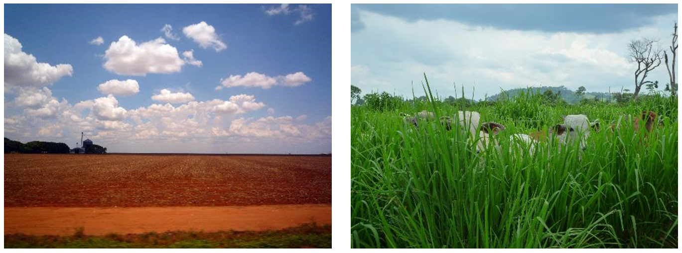
Post-deforestation land uses in the study region include intensive soy cultivation (left) and extensive cattle ranching (right). Images: Philippe Rufin

From a remote sensing perspective, separating cropland and grassland is challenging due to similar spectral signatures during most periods of the year. In certain periods however, differences in land surface phenology become apparent. We can investigate these differences by creating an intra-annual time series of Tasseled Cap Greenness (TCG).

Intra-annual time series of Tasseled Cap Greenness for 2010.

Let´s investigate differences between pastures and croplands over time. We collected 50 reference samples for pastures and 50 for cropland in the study region. We then extract the TCG value for all those locations in each of the time series bands. In a next step, we can create class-wise boxplots for each observation date. The boxplots reveal the land surface dynamics for each class.

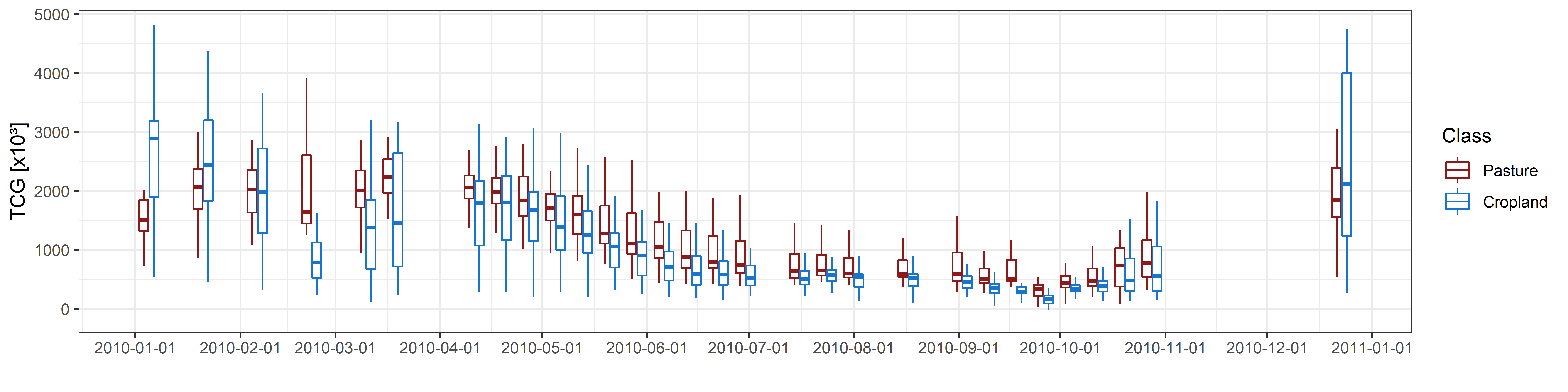
Boxplots showing the distribution of TCG for pastures (n = 50 samples) and cropland (n = 50 samples) across all observations of the year 2010.

Can you identify differences between the classes? Looking at the above graph suggests that croplands have a somewhat higher variability throughout the year, but on average, pastures show a slightly higher TCG. We can try to verify this by calculating descriptive statistics of all TCG observations in the year and then comparing those between the classes. Let´s take a look at the maximum, mean, minimum, and standard deviation of TCG throughout 2010.

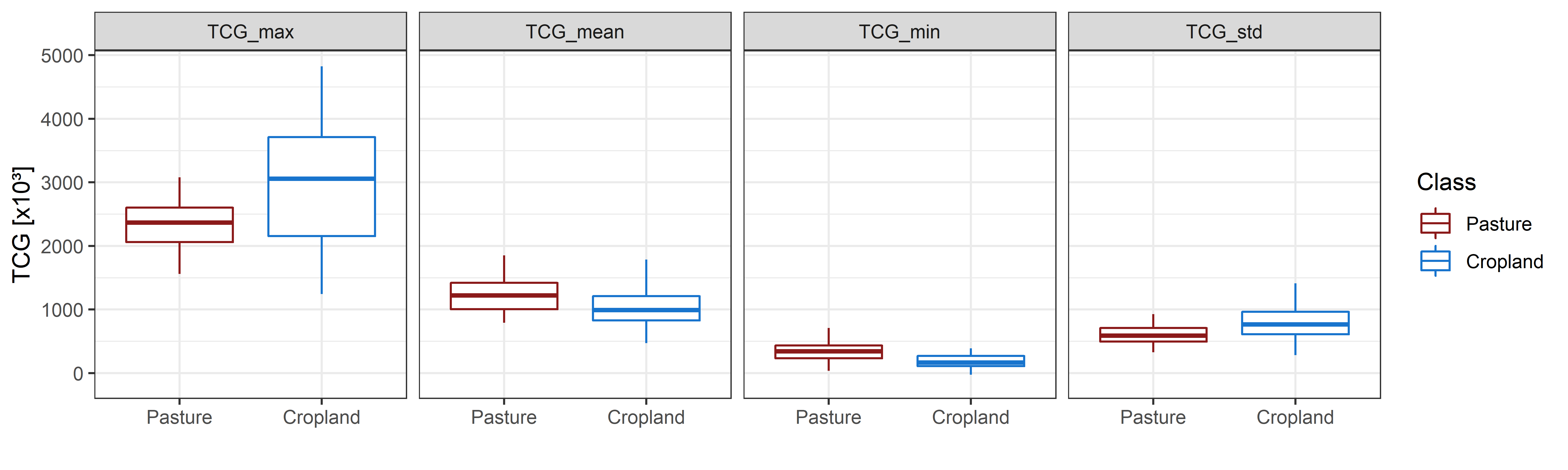
Boxplots showing the distribution of maximum, mean, minimum and standard deviation of TCG for pastures (n = 50 samples) and cropland (n = 50 samples) in 2010.

We can see that these “temporal statistics” can be useful to discriminate the two spectrally similar classes. Features combining the spectral appearance of a surface with its behaviour over time are increasingly popular in the remote sensing community. We refer to such features as spectral-temporal metrics (STM). STMs are descriptive statistics of the spectral behaviour over time. They provide an efficient means to capture seasonal variations of land surface dynamics, while reducing the impact of clouds and cloud-shadows as well as reducing the dimensionality of dense time series. STMs can be calculated from indices such as the NDVI or TC components, but also directly from spectral bands.

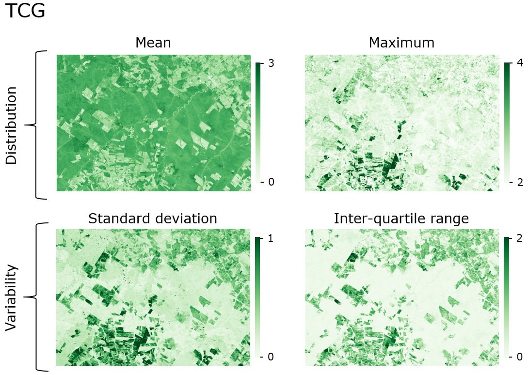
Exemplary metrics calculated from intra-annual time series of Tasseled Cap Greenness.

Different metrics might be more or less useful depending on the application. Good process understanding is key in finding out which STMs are relevant for the problem at hand. We should decide on the type of spectral information and a set of statistics (metrics) to compute. Providing such information to a classifier can enable the production of thematically detailed land cover maps over large areas, such as a pan-European land cover map.

Assignment

In this assignment, you will create STMs for forest type differentiation in the Carpathian study area. We will, once again, use the time series that you took for creating BAPs, complemented by your training data from session 3:

Preprocessed Landsat-7 and Landsat-8 band-wise (blue, green, …) surface reflectance time series from 2014 to 2016 ("/imagery/time-series")
Your training points (.gpkg) for deciduous, mixed, coniferous woody vegetation and all remaining land cover types
Pre-calculated STMs from the surface reflectance data covering all data between 2014-2016 ("/imagery/stm"). This includes the minimum (MIN), mean (MEA), maximum (MAX), 10th-, 25th-, 50th- (MED), 75th-, 90th-percentile (P10-P90), and standard deviation (STD)

1) Inspect the input data

Open a new QGIS project and inspect the pre-computed spectral-temporal metrics ("/imagery/stm"). Choose one indicator (e.g. Tasseled Cap Greenness) and load all layers. Make sure you understand what the metrics represent and discuss their meaning, robustness (e.g. against cloud contamination), and behavior over different land cover types within your group.

Next, compare the temporal behavior of the four classes, identify the main characteristics and differences. For this you can recycle the code from session 3 “3) Explore your training data”.

Two exemplary plots that could guide you in identifying key periods and metrics are shown below. For example, the first plot showing the spectral-temporal trajectories of the TCB suggests, that the three forest classes have different degrees of intra-annual variability (lowest for coniferous, highest for deciduous). Potentially, the standard deviation or inter-quartile range are good indicators of this.

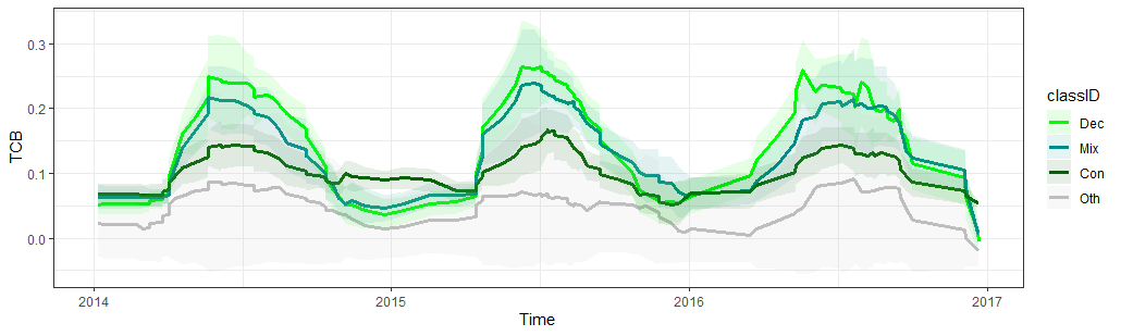
Spectral-temporal trajectory of the Tasseled Cap Brightness for the four different land cover classes

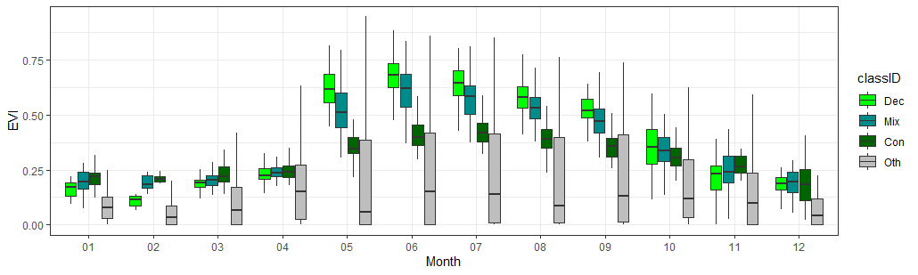
Monthly class-wise boxplots of the EVI aggregated between 2014-2016

Please record your insights as comments in your script and select at least 6 additional statistical metrics for different sub-periods in time that you believe capture the differences between the forest types and other land cover well.

Please note:

your “sub-periods in time” can e.g. cover the summer months (but using all data from the three years), single years
further below the page you find some code snippets that help you subset the time series into desired time chunks and calculate STMs only on these subsets
not all metrics you choose have to - or rather could - perfectly differentiate the classes. A good mixture of various feature/band and metric combinations are key in that regard.
‘extreme’ metrics such as the minimum or maximum often exhibit noise since bright cloud remnants or dark shadows that were not entirely removed during pre-processing tend to lie at the edge of the feature space (view e.g. 2014-2016_001-365_HL_TSA_LNDLG_BLU_MAX)

2) Compute additional spectral-temporal metrics

Based on your conceptual selection of additional STM candidates, let´s generate additional STMs from the time series stacks.

A number of summarizing functions can be applied directly to raster stacks (mean(), max(), min(), range()). If you want to calculate metrics other than those - or more generally: want to apply other functions to your rast-object -
you can either convert your raster into a matrix using as.matrix() or make use of terra’s built-in app-function. The below figure helps to understand how a three-dimensional raster stack is being transformed into a two-dimensional matrix.

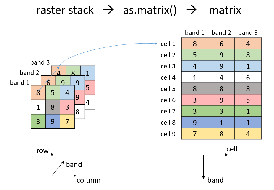
Schematic illstration of converting a raster stack to a matrix using the as.matrix() function.

Based on the resulting matrix, you can create temporal subsets by selecting the desired columns, and perform basic calculations using, e.g., apply(). Using apply(), the specified function is applied along the x-dimension (row-wise) of the 2D matrix, resulting in a single column matrix (i.e., a vector). This single column matrix can then be converted back into a 2D raster using the rast-function and specifying the raster properties (extent, CRS, …) based on your original raster object.

The following code template gives an example for computing the 10th percentile of the EVI around the peak-of-season DOYs. Note that computations can take several minutes.

# load the terra package
library(terra)

# read TCG time series stack (remember to set your working directory before)
evi <- rast('imagery/time-series/2014-2016_001-365_HL_TSA_LNDLG_EVI_TSS.tif')
tcb <- rast('imagery/time-series/2014-2016_001-365_HL_TSA_LNDLG_TCB_TSS.tif')

# retrieve temporal information from bandnames
library(lubridate)
datestring <- unlist(lapply(names(tcb), function(x) substr(x, 1, 8)))
dates <- as.POSIXlt(datestring, format = "%Y%m%d")

# on this date-object, we can perform logical operations
# for example, let's find the indices for the months June-August only
condition <- (year(dates) %in% 2014:2016) & (month(dates) %in% 6:8)

# --------------------------------------------------------------------
# Option 1) terra's convenient app-function
evi_p10 <- terra::app(evi[[which(condition)]], quantile, probs = c(.10), na.rm=T)
# plot result
plot(evi_p10)

# --------------------------------------------------------------------
# Option 2) convert raster subset to matrix
evi_matrix <- as.matrix(evi[[which(condition)]])
# calculate P10 across rows in matrix
evi_p10 <- apply(evi_matrix, 1, FUN=quantile, probs = c(.10), na.rm=T)
# write results to empty raster
evi_p10 <- terra::rast(nrows=nrow(evi), 
                            ncols=ncol(evi), 
                            crs=crs(evi), 
                            vals=evi_p10,
                            ext=ext(evi))
# plot result
plot(evi_p10)

Calculate your selected STMs and write them into your STM directory ("/imagery/stm").

Next session, we will use the BAPs and STMs you calculated in combination with your training data to classify the study area using Random Forest classification models.

Reading materials

For the next session, please read the following paper: Maxwell et al. (2018): Implementation of machine-learning classification in remote sensing: an applied review. International Journal of Remote Sensing 39(9), 2784-2817

In this review, Maxwell and colleagues outline the use of several machine learning classification algorithms for application in remote sensing. Please read the article and note questions and points to discuss. Feel free to omit the details of ANNs and boosted DTs. Please read the paper thoroughly, make sure you understand the underlying concepts and write down questions for the discussion in our next session. Try answer the following questions:

What is the motivation for this article?
What are the key differences between the presented classification algorithms from a user perspective?
What do the following terms refer to: “overfitting”, “imbalanced data”, “ensemble classifiers”, “parameter optimization”?

Recommended (voluntary) regarding ‘Random Forests’

Since we will have a particular focus on Random Forest classification next session, we provide you with (voluntary) book chapters introducing the concept of decision trees and bootstrap aggregation (bagging) - i.e. the architecture on which Random Forests are built upon:

Introductory level: James et al. (2013): An Introduction to Statistical Learning (with Applications in R). Chapter 8 Tree-Based Methods. Springer Texts in Statistics.

Advanced level: Hastie et al. (2009): The Elements of Statistical Learning. Chapter 15 Random Forests. Springer Series in Statistics.

We largely stick to a conceptual understanding of Random Forest (RF) classification. Please be guided by the following questions and write down any questions that come up during reading that we can discuss in the next session:

What is the basic architecture/structure of decision trees?
How does decision tree learning work? How are optimal splits defined?
What are the two layer of randomness in Random Forests?
How does bagging work?
Why do RFs only consider a subset of all features at each decision node?