Digital Numbers | TOA & BOA Reflectance

Learning goals

Calibrating optical imagery by converting Digital Numbers (DNs) to Top-Of-Atmosphere (TOA) reflectance
Compare TOA reflectance to atmospherically corrected data, i.e. Bottom-Of-Atmosphere (BOA) reflectance

Background

What is radiance / what are DNs?

Today we will be dealing with physical units, conversion, and data quality. Let´s kick it off with a short recap. Last session, you scaled the Landsat data using the sensor-specific calibration coefficients, by applying the following equation:

\[Reflectance = 0.00002 * DN - 0.1\]

But what are DNs? Optical Earth observing sensors, such as the ones on board the Landsat satellites, register radiance at the top of the atmosphere. Radiance is expressed in watt per steradian per square meter.

Storing data in radiance units is impractical and therefore sensors translate measured radiance into DNs. This means that the range of energy measured by the sensor is broken into distinct units (the DNs). Sensor-specific calibration determines the minimum and maximum amount of radiance that can be measured. The sensors capability to measure differences in energy. The sensitivity so to speak. DNs simply are the digital way to store this information and express the amount of radiance in relation to these sensor-specific calibration coefficients. The total number of possible DNs is what we refer to as the radiometric resolution of the sensor, the ability of a sensor to measure differences in incoming energy. The finer these differences can be, the more sensitive the sensor is and the better the radiometric resolution.

As an example, Landsat-4 , -5, and -7 worked with a radiometric resolution of 8-bit. This allows for 2^8, or 256 distinct DNs values. Why, you ask? We will answer this in the second section of today´s session. Now, Landsat-8 and -9 operate at 12-bit radiometric resolution. The actual data is ‘artificially’ quantized in 16-bit (simply because the common steps are 8, 16, 32, 64 bit). Using a 16-bit resolution, nuanced differences in light intensity can be distinguished even better, i.e. exactly 2^16, or 65,536 unique values.

library(terra)

# Define the number of bits
bit <- 4

# How many grey tones can we represent given bit?
print(paste0(bit, ' bits produce ', 2^bit, ' grey tones.'))

# Create a new raster with one line and 2^bit columns,
# whereas cell values are filled with a vector of numbers from 1 to 2^bit
r <- rast(nrows = 1, ncols = 2^bit, vals = c(1:2^bit))

# Plot the raster and assign grey-scale values to the cells
image(r, col = grey.colors(2^bit, start = 0, end = 1), main = paste0(bit, ' bit resolution'))

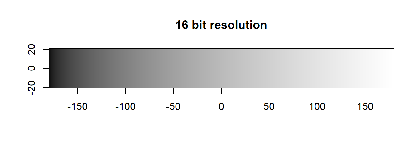
Let´s do the same with bit <- 16.

As already said, we will learn more on how we get these values in the next section, but for now let´s get back to converting our data from DNs to TOA, i.e. apply sensor calibration.

Digital Numbers (DNs) to Top-Of-Atmosphere (TOA)

As DNs are dependent on sensor calibration, identical radiance measurements can yield differing DNs across sensors. Since DNs are just used to store the data, they are physically not meaningful. We are interested in reflectance. Reflectance expresses the fraction of reflected radiance relative to the total incoming energy (i.e., from the sun), and thus ranges between 0 and 1. Many applications require data converted to reflectance and/or corrected for the influence of the atmosphere. The following steps are necessary to convert DNs into (atmospherically corrected) Bottom-Of-Atmosphere (BOA) reflectance:

Sensor calibration (DN to radiance)
Conversion to top-of-atmosphere (TOA) reflectance (radiance to TOA)
Atmospheric correction yielding bottom-of-atmosphere (BOA) reflectance (TOA to BOA)

A conversion of DNs into radiance can be easily undertaken. By accounting for sun-sensor-geometries and solar irradiance, we can easily infer top-of-atmosphere reflectance (TOA) from radiance. This facilitates, e.g., a comparison of measurements from different sensors.

Practically, this involves the linear scaling you already applied of the DN values using band-specific rescaling factors. For Landsat, this is achieved with a linear model, hence one factor is multiplicative, one is additive. Formulas are explained in the USGS guide for conversion to TOA Reflectance. With Landsat-8 Collection 2 data (this is not the case for all sensors!), we can use a single set of coefficients for all bands to convert DNs directly to TOA reflectance:

\(ρλ' = M_ρ * Q_{cal} + A_ρ\)

where

\(ρλ'\) = TOA planetary reflectance, without correction for solar angle.

\(M_ρ\) = Band-specific multiplicative rescaling factor from the metadata.

\(Q_{cal}\) = Quantized and calibrated standard product pixel values (DN).

\(A_ρ\) = Band-specific additive rescaling factor from the metadata.

In a next step, we can correct for solar angle during image acquisition.

\(ρλ = \frac{ρλ'}{cos(θ_{SZ})} = \frac{ρλ'}{sin(θ_{SE})}\)

where

\(ρλ\) = TOA planetary reflectance corrected for solar angle.

\(θ_{SZ}\) = Local solar zenith angle, whereas \(θ_{SZ} = 90° - θ_{SE}\).

\(θ_{SE}\) = Local sun elevation angle.

TOA to BOA

Atmospheric correction is the final step towards obtaining comparable measurements of the Earth’s surface. By applying atmospheric correction, we (theoretically) eliminate the influence of the atmosphere on the measured signal. We therefore call the product “Bottom-Of-Atmosphere” (BOA) reflectance, as it comes closest to ground-based measurements. A multitude of algorithms and associated software packages exist for applying atmospheric correction and Landsat imagery can also be directly ordered as atmospherically corrected data from the USGS EarthExplorer.

Assignment

During this assignment you will learn how to convert Landsat-8 Collection 2 DNs to TOA reflectance, and then identify and compare the spectral appearance of different land cover types in TOA versus BOA imagery.

Today, we will use the summer scene, i.e. acquired on the 16th of July 2014:

Before we can start, use your workflow from last session to …

… read in the spectral bands into a raster stack
… rename the bands c("BLU", "GRN", "RED", "NIR", "SW1", "SW2")
… reproject the stack onto the CRS and extent of reference.tif or your output stack from last session

Do this for both summer images, i.e. processing levels:

LC08_L1TP_189025_20140716_20200911_02_T1 = DN/TOA
LC08_L2SP_189025_20140716_20200911_02_T1 = BOA

1) DN to TOA conversion

Familiarize yourself with the L1TP data and specifically take look at the metadata file (LC08_L1TP_..._MTL.txt) and the information provided within. As mentioned above, we need the calibration coefficients to scale our data according to your needs. Last session, we provided you with the two factors needed to scale from DN to TOA. Although these are currently identical for all Landsat-8 bands, this is not the case for Landsat-7 and might change in the future. To be on the safe side and simplify the workflow, we are going to automatically extract the conversion factors from the .txt file in R.

Comprehend the following function to extract the conversion factors, and complement it to also extract the sun elevation from the metadata.

# get conversion factors
get_conv_val <- function(inp_dir, band_range="[2-7]"){
  # retrieve metadata file within folder
  mtl <- list.files(inp_dir, pattern='MTL.txt$', full.names=T)
  # read file into table
  mtl_txt <- read.delim(mtl, sep = '=', stringsAsFactors = F, header = FALSE) 
  names(mtl_txt) <- c("VAR", "VAL")  # add header
  # get conversion factors according to specified band range
  REFLECTANCE_MULT_BAND <- as.numeric(mtl_txt[grep(paste0("REFLECTANCE_MULT_BAND_", band_range), 
                                                   mtl_txt$VAR),][,2])
  REFLECTANCE_ADD_BAND <- as.numeric(mtl_txt[grep(paste0("REFLECTANCE_ADD_BAND_", band_range), 
                                                   mtl_txt$VAR),][,2])
  # get sun elevation during acquisition
  SUN_ELEVATION <- 

  return(list(REFLECTANCE_MULT_BAND, REFLECTANCE_ADD_BAND, SUN_ELEVATION))
}

Retrieve the needed coefficients for DN to TOA conversion from the metadata and store them as variables
Convert the DN image stack to TOA reflectance with the correction for the sun angle (see “Background” section)

Note: SUN_ELEVATION in the metadata file is reported in degrees. The sin() function expects that angles are provided in radians. Hence, you need to convert SUN_ELEVATION into radians, using this helper function:

  # Helper-function to convert degrees to radians
  deg2rad <- function(deg){ (deg * pi) / (180) }

Inspect your result and then write the scaled TOA stack to disk using the GTiff format.

2) Compare TOA to BOA

Next, we want to compare the TOA and BOA imagery and assess the differences in the spectral signature between surface and top-of-atmosphere reflectance. Accordingly, we first repeat the above process for the L2SP product, thus:

Convert (or in this case rather, rescale) values to reflectance:
- REFLECTANCE_MULT_BAND = 2.75e-05
- REFLECTANCE_ADD_BAND = -0.2
Export stack to GeoTIFF

Next, open the BOA and the TOA file in QGIS and visually assess the differences in the spectral signature between the SR and TOA files. Use the info tool in graph view to plot the spectral signatures of each of the following land cover types:

Forest
Open soil
Water

In your R script, add comments for the following:

Briefly summarize the spectral appearance of the different land cover types.
What are the most evident differences between TOA and BOA reflectance spectra?