Course preparation: R basics

Here, we aim to provide a brief overview on the basics of R, which is supposed to refresh your knowledge and help you to identify topics worth revisiting. You are encouraged to refresh your knowledge from the module “Quantitative Methods for Geographers” as well as learn from online resources we list at the bottom of this page.

Operators

R is an interpreted programming language which means users can execute commands directly in the console without having to compile sourcecode. You can use R as a simple calculator using arithmetic operators and mathematical functions which are then evaluated directly. For example:

# A simple calculation
2*(1+4)

# abs() returns absolute values
abs(-2)  

# sqrt() returns the squareroot 
sqrt(pi)  # Note: 'pi' is a predefined constant

## [1] 10
## [1] 2
## [1] 1.772454

To list the defined operators used by R, simply type ?Syntax into the console. This includes the arithmetic operators

addition + and subtraction -
multiplication * and division /
exponentiation ^ or **

as well as logical operators

less than < / greater than >
less than or equal to <= / greater than equal to >=
equal to ==
not equal to !=
or |
and &

The concept of logical operators is to allow a program to make a decision based on (multiple) conditions. A condition can be evaluated to be either TRUE or FALSE (see ?Logic). For example:

2 > 5

## [1] FALSE

They are often used in combination with control statements such as the conditional if...else statement which are mentioned below. But first back to basic functions: R also comes with a whole set of mathematical functions including

trigonometric functions sin(), cos() and tan()
exponential function exp()
statistical metrics like min(), max(), median()

to name just a very few of them. Functions in R provide information on how to use them. If you need help with a function, type in help(name_of_function) or simply ?name_of_function to display the correct usage and syntax of a function.

Objects

Everything in R we assign to a variable is an object. We can assign objects in R with the <- operator (i.e. an arrow), e.g. x <- 2. Commonly, other languages use = which also works in R, however it is definitely good practice to use the <- operator in R.

# Assign object 'x' a value of 2
x <- 2  
# <- assigns the value, but does not print the result to console

# Assign  another variable 'y' ...
y <- 5

# Store the product of x and y in a new object 'z'
z <- x*y  

# Print z
print(z)

## [1] 10

Assigned variables are stored in the environment or workspace of our session and can be listed by calling the ls() function.

Data Types and Data Structures

The basic data types in R comprise:

Character (or String): sensor <- 'Landsat-8'
Integer: n_bands <- 11L (the L tells R it is an integer, otherwise it is interpreted as numeric)
Numeric (or Float): lambda_red <- 0.662
Logical (or Boolean): sun_synchronous <- TRUE or sun_synchronous <- T
Factors: agency <- factor('NASA',levels=c('NASA','ESA','INPE'))

Understanding data types is important for a variety of reasons. For instance, later in the course we will manipulate large rasters of remotely sensed reflectance data which may be stored as floating point numbers between 0 and 1. However, storing raster matrices as floats on disk requires more memory as compared to using an integer format. It can therefore be handy to transform data into integer prior to saving it to disk.

For now, let us just keep in mind that there are different data types and if we now want to store not just a single value into a variable but a whole set of data, we need to undertstand the different data structures available in R:

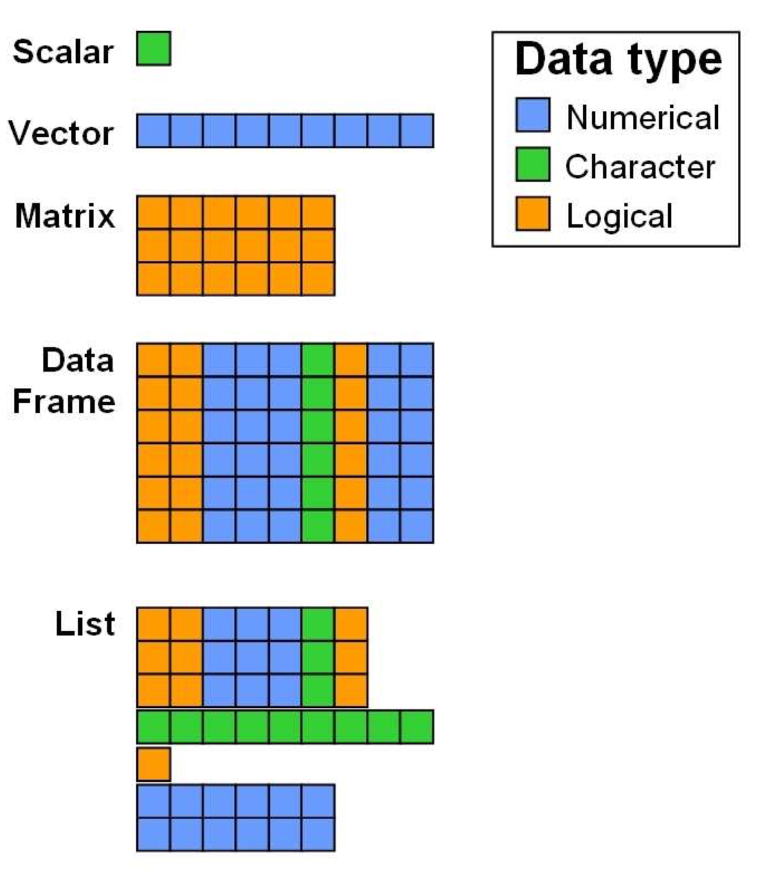
Data Structures in R (from Zimmermann & Steinmann 2006)

As you can see in the figure above, a variety of data structures exist in R, which either allow for storing different data types simultaneously (data frames, lists), or only one datatype (scalars, vectors, matrices). Note, that the colors representing the data types are only chosen for vizualisation purposes: It does not mean that matrices or vectors can only store values of type logical or numeric, but only data of the same type.

Vectors

A vector in R can be created using a variety of functions. The most basic function is the c()-function, where ‘c’ stands for concatenate.

# Create a vector of numbers
a <- c(2, 4, 8, 16, 32)

# Print vector a in console
print(a) 

# cat-function: Similar to print, outputs the objects, concatenating the representations
cat('vector a:', a)

## [1]  2  4  8 16 32
## vector a: 2 4 8 16 32

Let`s see what happens when we mix numeric values with strings and combine them into a vector.

b <- c(2, 4, 8, 16, 32, 'Landsat', 'Sentinel-2')
print(typeof(b))

## [1] "character"

Our vector was automatically cast to character. This is because R will try and convert a smaller data type into a larger one to avoid data loss (here from numeric to character). The strings (Landsat and Sentinel-2) in vector b cannot be cast to numeric, however we can very well transform a numeric 2 into a string '2'. Be aware of this behaviour and use other data structures if needed.

Back to vector creation. Instead of having to type in sequences or replicates manually by hand, R provides the functions seq() and rep().

# Create a numeric sequence and store in object s
s <- seq(from=1, to=365, by=1)  # or simply s <- seq(1, 365, 1)
cat('Length of s:', length(s))

# Alternatively use (always with by=1):
s <- c(1:365)

# We may want to repeat a value n times... 
r <- rep(1, 5)
print(r)

# ...or repeat a sequence 
r <- rep(seq(2, 8, 2), 3)
print(r)

# ...or repeat each entry in a sequence 
r <- rep(seq(2, 8, 2), each=3)
print(r)

## Length of s: 365[1] 1 1 1 1 1
##  [1] 2 4 6 8 2 4 6 8 2 4 6 8
##  [1] 2 2 2 4 4 4 6 6 6 8 8 8

Matrices and Arrays

Creating matrices and arrays is just as easy as creating vectors. Matrices are just 2-dimensional arrays with a specified number of rows and columns. All columns in a matrix must have the same data type (e.g., numeric, character) and must be of equal length.

# Creates empty matrix of size 5x2
m1 <- matrix(data=NA, nrow=5, ncol=2) 
print(m1)

# Creates matrix of size 5x2 containing a numeric vector
m2<- matrix(data=c(1:10), nrow=5, ncol=2) 
print(m2)

# Can you describe what byrow=T does?
m3 <- matrix(data=c(1:10), nrow=5, ncol=2, byrow = T) 
print(m3)

##      [,1] [,2]
## [1,]   NA   NA
## [2,]   NA   NA
## [3,]   NA   NA
## [4,]   NA   NA
## [5,]   NA   NA
##      [,1] [,2]
## [1,]    1    6
## [2,]    2    7
## [3,]    3    8
## [4,]    4    9
## [5,]    5   10
##      [,1] [,2]
## [1,]    1    2
## [2,]    3    4
## [3,]    5    6
## [4,]    7    8
## [5,]    9   10

Arrays are similar to matrices, but can have more than two dimensions, as specified in the dim argument.

# Create array of two 4x3 matrices
a <- array(data=c(1:12), dim=c(4,3,2)) 
print(a)

## , , 1
## 
##      [,1] [,2] [,3]
## [1,]    1    5    9
## [2,]    2    6   10
## [3,]    3    7   11
## [4,]    4    8   12
## 
## , , 2
## 
##      [,1] [,2] [,3]
## [1,]    1    5    9
## [2,]    2    6   10
## [3,]    3    7   11
## [4,]    4    8   12

In R, basic mathematical operations may be used to manipulate arrays. This can be used to add, subtract, multiply or divide a constant from every element in the array.

# Create array of one 4x3 matrices
a <- array(data=c(1:9), dim=c(4,3,1)) 

a2 <- a * 10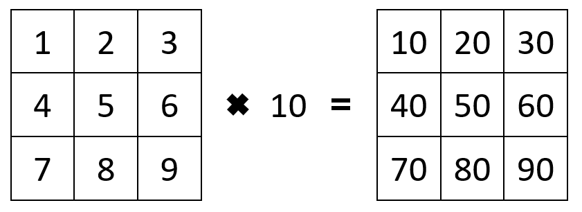

An entire array can be scaled by multiplying it with a constant

We can also use these operations on multiple arrays of the same size. This array arithmetic works element-wise. For example multiplying two arrays together, the first element element of the first array is multiplied by the first element of the second array, and so on. Note: while not needed in this course, R is also capable of performing matrix algebra using these operators.

# Create two arrays each of one 4x3 matrices
a1 <- array(data=c(1:9), dim=c(4,3,1)) 
a2 <- array(data=c(1:9), dim=c(4,3,1)) 

a3 <- a1 * a2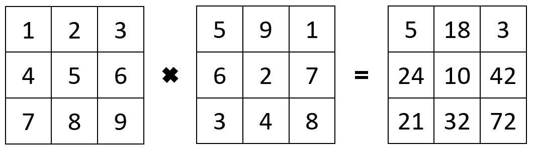

Multiplying two arrays of the same shape together results in element-wise multiplication

Matrices are very important structures when working with remote sensing data, as this is how images are represented numerically. We will extensively make use of the raster package throughout the course where a lot of the handling is done for us, however sometimes we need to manipulate image data with more advanced techniques and it is therefore crucial to understand the underlying data structure.

Data Frames and Lists

Generally speaking, a data.frame is a list of vectors of equal length, which can have varying data types.

# Create data.frame with four columns of different data types
df <- data.frame(sensor = c('Landsat-5 TM', 'Landsat-7 ETM+', 'Landsat-8 OLI-TIRS'), 
                 n_bands = c(7, 8, 11), 
                 active = c(F, T, T), 
                 launched = c(1984, 1999, 2013))
print(df)

##               sensor n_bands active launched
## 1       Landsat-5 TM       7  FALSE     1984
## 2     Landsat-7 ETM+       8   TRUE     1999
## 3 Landsat-8 OLI-TIRS      11   TRUE     2013

The top line of the data.frame is the header, describing the column names. Each entry is called a cell and may be indexed (accessed) individually. We will see how this works in a moment.

Lastly, let us have a look at lists. Lists are objects that can contain elements of different types – vectors, string scalars, matrices, functions or yet another list. Hence, a list is a generic vector containing other objects. The dimensions of the elements to be included must not be identical, which gives us additional flexibility to integrate heterogeneous datasets. A list can be created using the list() function:

# Store the matrix, array and vector in a list
l <- list(m3, a, df)
print(l)

## [[1]]
##      [,1] [,2]
## [1,]    1    2
## [2,]    3    4
## [3,]    5    6
## [4,]    7    8
## [5,]    9   10
## 
## [[2]]
## , , 1
## 
##      [,1] [,2] [,3]
## [1,]    1    5    9
## [2,]    2    6    1
## [3,]    3    7    2
## [4,]    4    8    3
## 
## 
## [[3]]
##               sensor n_bands active launched
## 1       Landsat-5 TM       7  FALSE     1984
## 2     Landsat-7 ETM+       8   TRUE     1999
## 3 Landsat-8 OLI-TIRS      11   TRUE     2013

As the print results suggests, our three objects are now stored at locations [[1]], [[2]] and [[3]]. We may want to access these list elements and cells therein individually. This brings us to the next topic - indexing.

Indexing

So how do we access values in vectors, data.frames or the elements in the list we just created? Each element is assigned an index (i.e. a positive integer) which we can retrieve by addressing these indices. This is achieved using square brackets and a given index location(s).

b <- c(2, 4, 8, 16, 32, 64, 128, 256)

# Retrieve the 4th value of b
b[4]  

# Retrieve value 1, 2, and 3
b[1:3]

## [1] 16
## [1] 2 4 8

Use a vector to select certain positions:

# Retrieve value 1, 3, 5, and 7 of b
b[c(1, 3, 5, 7)]

## [1]   2   8  32 128

Manipulate entries:

# Set the first value in b to 0
b[1] <- 0 
print(b)

## [1]   0   4   8  16  32  64 128 256

For lists, one generally uses [[ to select any single element, whereas [ returns a list of the selected elements.

# [[]] returns element 1 in its original data type
typeof(l[[1]]) 

# [] returns a list containing element 1
typeof(l[1]) 

# Create a new object containing element 1
object_l <- l[[1]] 

# Create a new object containing cell [4,2] of element 1
cell_l <- l[[1]][4,2]

## [1] "integer"
## [1] "list"

We may also use the $ operator to access specific elements (in lists) or columns (in data frames), given that names were assigned. For example:

names(l) # Currently, our list does not have names...
names(l) <- c('matrix', 'array', 'df') #... names() can be used to assign element names
print(l$df)

print(df$n_bands)

## NULL
##               sensor n_bands active launched
## 1       Landsat-5 TM       7  FALSE     1984
## 2     Landsat-7 ETM+       8   TRUE     1999
## 3 Landsat-8 OLI-TIRS      11   TRUE     2013
## [1]  7  8 11

If you are uncertain about the characteristics of an object, you may use additional functions to investigate its attributes. Good examples are:

str(): structure of an object
length(): number of elements in one-dimensional objects or lists
nrow(), ncol(): number of rows or columns in 2-dimensional objects (df or matrix)
class(), typeof(): class or type of an object
names(): retrieve column names of df, or element names of list

Missing Values

Often our data has missing entries. For illustration, think of a vector of temperature measurements where due to measurement error we miss an entry now and then. For completeness, those are not just excluded but may often be represented by a certain value, e.g. -9999. In R missing values can be set to the logical constant NA (Not Available).

Let us consider an vector of hourly temperature measurements where -9999 in fact was used to represent erroneous measurements:

t_hourly <- c(10.1, 8.6, 8.2, 7.2, 6.8, -9999, 8.2, 9, 9.5, 10.5, -9999, 9.9, 9.7, 8, 7.7, 7.1, 6.8, 5.8, 5.2, 4.2, 4.0, 4.1, 4.2, 3.8)

# Calculate daily mean temperature
mean(t_hourly)

## [1] -826.6417

These measurements exhibit two invalid temperature values of -9999. Accordingly, the calculated mean is not of value to us. We need to flag these entries as invalid or more generally not available NA:

# Use indexing with logical condition
t_hourly[t_hourly == -9999] <- NA

# ...ifelse to manipulate array: ifelse(condition, TRUE, FALSE)
t_hourly <- ifelse(t_hourly == -9999, NA, t_hourly)

# mean() will yield NA as soon as one NA value appears unless...
mean(t_hourly)

# ... we specify na.rm = True to ignore missing values:
mean(t_hourly, na.rm = T)

## [1] NA
## [1] 7.209091

There are often various ways to achieve what we want, the best way largely depends on how we want to proceed with our data. Here are more examples to do the same:

t_hourly <- c(10.1, 8.6, 8.2, 7.2, 6.8, -9999, 8.2, 9, 9.5, 10.5, -9999, 9.9, 9.7, 8, 7.7, 7.1, 6.8, 5.8, 5.2, 4.2, 4.0, 4.1, 4.2, 3.8)

# Use only the entries that are not -9999...
mean(t_hourly[t_hourly != -9999])

# ...or use non-NAs after assigning NA to -9999
t_hourly[t_hourly == -9999] <- NA
mean(t_hourly[!is.na(t_hourly)])

## [1] 7.209091
## [1] 7.209091

Flow Control

Often we want code to be executed only when certain conditions are met (conditional statements) or repeat a certain chain of commands in order (repeating operations). For conditional statements, the most commonly used approach are if statements which are based on boolean logic. Accordingly, it is evaluated if a condition is TRUE or FALSE and the following code block will therefore be executed (TRUE) or not (FALSE).

if-statements

The basic form of an if statement could be as follows:

# Reclassify an image based on a certain NDVI threshold, after a sanity check if the threshold is valid
ndvi_threshold <- 0.8

if (ndvi_threshold > 1 | ndvi_threshold < -1) {  # i.e. if NDVI larger 1 OR smaller -1
  print('Invalid NDVI threshold provided. Must be in range -1 to 1.')
  
} else {
  print('Valid NDVI threshold. Continue processing ...')
  # Additional code to be executed follows here ....
}

## [1] "Valid NDVI threshold. Continue processing ..."

Above we already used the vectorized version ifelse() which for instance allowed us to manipulate out vector of temperature records:

t_hourly <- ifelse(t_hourly == -9999, NA, t_hourly)  # ifelse(condition, TRUE, FALSE)

Loops

for loops can be used to iterate over items and repeatingly execute code blocks:

# Generate sequence of integers from 1 to 10 with a step size of 1
v <- seq(1, 10, 1)

# Iterate over each entry in v and print
for (item in v){
  print(item)
}

## [1] 1
## [1] 2
## [1] 3
## [1] 4
## [1] 5
## [1] 6
## [1] 7
## [1] 8
## [1] 9
## [1] 10

while repeatedly evaluates a condition and executes commands until the final condition is fulfilled.

# Assign integer to v
v <- -3

# Adds +1 to v and then prints until v > 2
while (v <= 2) {
  v <- v + 1
  print(v)
}

## [1] -2
## [1] -1
## [1] 0
## [1] 1
## [1] 2
## [1] 3

Note that loops should be avoided in higher-level languages such as R or Python where possible because they tend to make the programs run slower than when using in-built vectorized functions. For example, calculating the sum over a vector may be calculated as follows:

s <- seq(1, 10, 0.5)

s_sum <- 0
for (i in s){
  s_sum <- s_sum + i
}
print(s_sum)

## [1] 104.5

Much more elegant and faster (think of manipulating large datasets) is to use

s_sum <- sum(s)
print(s_sum)

## [1] 104.5

Functions

R allows for user-specified functions which comes in handy whenever a certain computation needs to be repeated or generalized. Generally, a function is a set of statements organized together to perform a specific task. Using functions greatly enhances code structure as it improves the clarity and readability of your script.

Function arguments are provided in round () brackets. Between {} stands the function body which contains the collection of statements. return() is used to define the output of a function. A function may be as simple as a print statement without any objects to be returned.

A function object is defined with the function() call:

# Basic function
printer <- function(){
  print('Hello World!')
}

printer()

## [1] "Hello World!"

Another example where we want the function to calculate the NDVI for a given pair of reflectance values in the red and near-infrared region of the spectrum:

# Function to calculate the NDVI
calc.ndvi <- function(red, nir, scale_factor=1){
  ndvi <- (nir-red)/(nir+red)
  return(ndvi*scale_factor)
}

p_red <- 0.2
p_nir <- 0.8

ndvi <- calc.ndvi(p_red, p_nir)
print(ndvi)

## [1] 0.6

Here, red and nir are obligatory arguments that the user has to specify while scale_factor is optional as such that it has a default value which may or may not be altered.

Tutorials

We here covered only very basic aspects of R. At this stage, we did not cover advanced data wrangling using packages such as tidyr or dplyr, or look into advanced plotting with ggplot2. Please follow one or several tutorials to revisit and amend your knowledge:

General tutorials:

Graphics & visualization:

Geodata processing:

Coding style

A few basic rules apply to coding in R. Here is a short summary of Hadley Wickham´s style guide:

Regularly save your progress.
Script names should be meaningful and end in ‘.R’.
Comment (#) your code & separate it into readable chunks.
Try to limit your code to 80 characters per line.
Variable and function names should be lowercase.
Variable names should be nouns and function names verbs.
Place spaces around operators (=, +, -, <-, etc.) and after commas.
Use <-, not =, for assignment.

An example:

######################################################
# Creating random data and a correlated response 
# Author, 2020

# Load all required packages
library(ggplot2)

## Warning: package 'ggplot2' was built under R version 4.1.2

# Create random data
x <- runif(50, 0, 2)

# Build function to simulate response
create.response <- function(x){x + rnorm(50, 0, 0.2)}

# Apply function to random data
y <- create.response(x)

# Make a dataframe
data <- data.frame('x' = x, 'y' = y)

# Plot the simulated dataset
ggplot(data, aes(x = x, y = y)) +
  geom_point()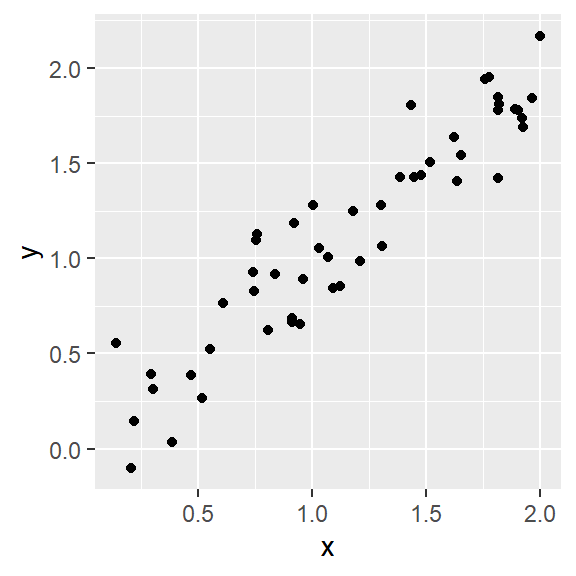

# Investigate correlation in the data
cor(data$x, data$y)

## [1] 0.9463074

Help!

If you get stuck while programming, there are plenty of things you can do:

Seek the function´s help page (i.e. highlight the function and hit F1)
Search your problem or error message
Ask your colleagues
Use the moodle course forum
Check forums (e.g., StackOverflow)