Training data
Learning goals
- Understand how forest types differ spectrally
- Gather training data for a forest type classification
Background
Collecting training information is an essential step on your way to a classified map. The training pixels should be considered representative for the classes you want to map, as classification algorithms determine class labels for unknown pixels based on their similarity to the training dataset.
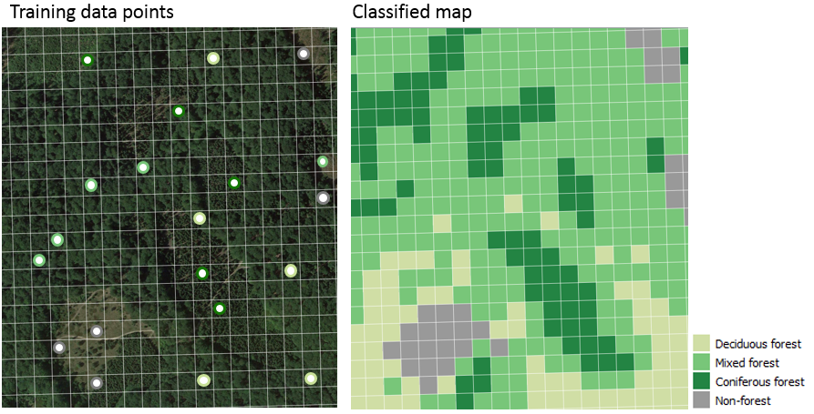
Training points for forest type classification and the resulting classification map output
Collecting training data is time consuming, regardless if you are collecting in the field or digitally. Small conceptual mistakes may require a revision of your training dataset. Consequently, your training data collection approach should be thoroughly planned before you start. Consider the following points:
A precise and robust definition of your target classes based on the study region characteristics and research questions is key. Targeting a high thematic detail is beneficial, but spectral(-temporal) similarities between classes might pose limitations to a robust distinction of classes, such as tree species or crop types. In such cases, it is advised to think about a hierarchical structure to aggregate similar classes into more general classes, such as tree species into forest types, or crop types into annual / perennial croplands. Keep the goal/questions posed in mind.
Include high quality reference information where possible. Can we find additional datasets that guide our interpretation? Is any very high resolution (VHR) imagery available? Google Earth is a valuable source of VHR imagery, but it is critical to account for the exact acquisition date, which you can identify with the “historic image” tool. When using other datasets, it is important to understand the relative geometric accuracies as well.
Training data must be representative. A models performance - e.g. on differentiating land cover classes - is largely bound by the data it has been trained on. Make sure the variance within classes and (often) marginal differences between classes is adequately captured in the data. For example, deciduous forest can “look” very differently in their spectral behaviour and the variance should be included in the data. This also links to the next point ….
Stratify your data collection - spatially, spectrally (and temporally) Random point sampling is unlikely to be the best option for training data collection (unlike collecting independent validation data), as we might want to train small classes that are unlikely to be adequately captured with a random sample. Manual selection of training points is often advised to circumvent this problem. Cover your study area well. The image below shows the spatial distribution of six training datasets collected during an earlier iteration of the course. Notice that some training points cluster in a subset of the study region. Ideally, however, training data should be well distributed across the study region to cover regional biophysical variability, such as different soil types, weather patterns, or topography.
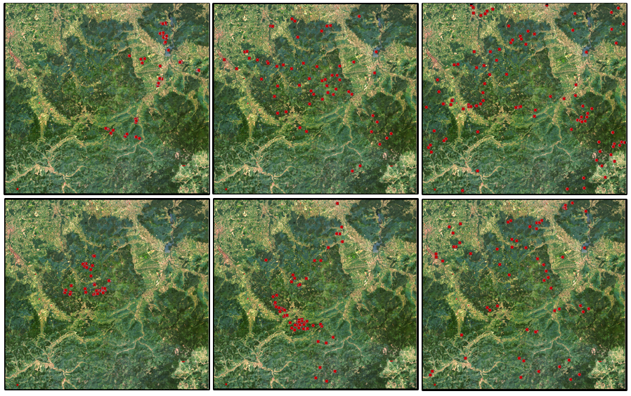
Spatial distribution of six training datasets
Another note:
- The classification algorithm of your choice might have specific requirements regarding the training data, e.g., concerning the number of samples, their distribution in the spectral feature space, or their purity (pure vs. mixed pixels). We will discuss these aspects later in the course when we apply machine learning to build classification models.
Assignment
This assignment has two larger aims. First, you will learn how broad forest types appear spectrally in images over the course of the image time series. Second, you will use this knowledge to collect training data for a broad forest type classification. We provided you with forestry data to find representative sample pixels in QGIS. We will use the data you generate in this assignment in Session 5 for training a model to classify the imagery in forest types. Accordingly, we must work thoroughly during our collection for the classification to turn out nicely.
First, get acquainted to the datasets:
…vector/BDL_stand-species_EPSG3035.gpkg: The dataset from last week: Forestry data collected in 2015. Recall the attributes most important to us:
| Attribute field | Definition | Class |
|---|---|---|
| species_en | Dominant genus in each stand | Ash, Beech, Fir, Spruce… |
| part_cd | Share of this genus within the stand | 0 – 100 (in %) |
| spec_age | Average age of the trees in this stand | Age in years |
| type | “species_en” reclassified into coniferous and deciduous | 1 = deciduous, 3 = coniferous |
…imagery/BDL_stand-species_type.tif: The rasterized
version of the attribute type in
“BDL_stand-species_EPSG3035.gpkg”
…vector/landsat_30m_grid: A .gpkg and
.kml file (Google Earth), which will help you to accurately
delineate the Landsat pixel extent for training data collection.
…imagery/time-series/2014-2016-4D-TSS.vrt: The
Virtual Format is a GDAL data
format that allows to combine multiple raster datasets into a single
file .vrt. The combination can be spatially (a mosaic of
smaller images), spectrally/temporally (multiband) or both. In our case,
it allows to access the time series of all spectral bands and indices
from a single file.
1) Preparing the training data collection
Visualize and arrange all aforementioned datasets in QGIS for training data collection:
2014-2016-4D-TSS.vrt: Find a good false-color representation of the Landsat bands and/or Tasseled Cap to highlight differences in vegetation. Find one (almost) cloud-free summer and winter/spring. If needed, recap and explore common settings here and here.BDL_stand-species_EPSG3035.gpkg: Visualize the different tree genera and/or the share of this genus within the stand.BDL_stand-species_type.tif- Load a high-resolution background layer into QGIS. You can add
background layers (
XYZ Tiles) from various sources, e.g. Google Satellite or OpenStreetMap, to QGIS. The following can be pasted into the Python console in QGIS to add a whole variety of them to your QGIS application:
Click here to view the python code and paste into python console in QGIS
# Sources
sources = []
sources.append(["connections-xyz","Google Maps","","","","https://mt1.google.com/vt/lyrs=m&x=%7Bx%7D&y=%7By%7D&z=%7Bz%7D","","19","0"])
sources.append(["connections-xyz","Google Satellite", "", "", "", "https://mt1.google.com/vt/lyrs=s&x=%7Bx%7D&y=%7By%7D&z=%7Bz%7D", "", "19", "0"])
sources.append(["connections-xyz","Google Terrain", "", "", "", "https://mt1.google.com/vt/lyrs=t&x=%7Bx%7D&y=%7By%7D&z=%7Bz%7D", "", "19", "0"])
sources.append(["connections-xyz","Google Terrain Hybrid", "", "", "", "https://mt1.google.com/vt/lyrs=p&x=%7Bx%7D&y=%7By%7D&z=%7Bz%7D", "", "19", "0"])
sources.append(["connections-xyz","Google Satellite Hybrid", "", "", "", "https://mt1.google.com/vt/lyrs=y&x=%7Bx%7D&y=%7By%7D&z=%7Bz%7D", "", "19", "0"])
sources.append(["connections-xyz","Stamen Terrain", "", "", "Map tiles by Stamen Design, under CC BY 3.0. Data by OpenStreetMap, under ODbL", "http://tile.stamen.com/terrain/%7Bz%7D/%7Bx%7D/%7By%7D.png", "", "20", "0"])
sources.append(["connections-xyz","Stamen Toner", "", "", "Map tiles by Stamen Design, under CC BY 3.0. Data by OpenStreetMap, under ODbL", "http://tile.stamen.com/toner/%7Bz%7D/%7Bx%7D/%7By%7D.png", "", "20", "0"])
sources.append(["connections-xyz","Stamen Toner Light", "", "", "Map tiles by Stamen Design, under CC BY 3.0. Data by OpenStreetMap, under ODbL", "http://tile.stamen.com/toner-lite/%7Bz%7D/%7Bx%7D/%7By%7D.png", "", "20", "0"])
sources.append(["connections-xyz","Stamen Watercolor", "", "", "Map tiles by Stamen Design, under CC BY 3.0. Data by OpenStreetMap, under ODbL", "http://tile.stamen.com/watercolor/%7Bz%7D/%7Bx%7D/%7By%7D.jpg", "", "18", "0"])
sources.append(["connections-xyz","Wikimedia Map", "", "", "OpenStreetMap contributors, under ODbL", "https://maps.wikimedia.org/osm-intl/%7Bz%7D/%7Bx%7D/%7By%7D.png", "", "20", "1"])
sources.append(["connections-xyz","Wikimedia Hike Bike Map", "", "", "OpenStreetMap contributors, under ODbL", "http://tiles.wmflabs.org/hikebike/%7Bz%7D/%7Bx%7D/%7By%7D.png", "", "17", "1"])
sources.append(["connections-xyz","Esri Boundaries Places", "", "", "Requires ArcGIS Onlinesubscription", "https://server.arcgisonline.com/ArcGIS/rest/services/Reference/World_Boundaries_and_Places/MapServer/tile/%7Bz%7D/%7By%7D/%7Bx%7D", "", "20", "0"])
sources.append(["connections-xyz","Esri Gray (dark)", "", "", "Requires ArcGIS Onlinesubscription", "http://services.arcgisonline.com/ArcGIS/rest/services/Canvas/World_Dark_Gray_Base/MapServer/tile/%7Bz%7D/%7By%7D/%7Bx%7D", "", "16", "0"])
sources.append(["connections-xyz","Esri Gray (light)", "", "", "Requires ArcGIS Onlinesubscription", "http://services.arcgisonline.com/ArcGIS/rest/services/Canvas/World_Light_Gray_Base/MapServer/tile/%7Bz%7D/%7By%7D/%7Bx%7D", "", "16", "0"])
sources.append(["connections-xyz","Esri National Geographic", "", "", "Requires ArcGIS Onlinesubscription", "http://services.arcgisonline.com/ArcGIS/rest/services/NatGeo_World_Map/MapServer/tile/%7Bz%7D/%7By%7D/%7Bx%7D", "", "12", "0"])
sources.append(["connections-xyz","Esri Ocean", "", "", "Requires ArcGIS Onlinesubscription", "https://services.arcgisonline.com/ArcGIS/rest/services/Ocean/World_Ocean_Base/MapServer/tile/%7Bz%7D/%7By%7D/%7Bx%7D", "", "10", "0"])
sources.append(["connections-xyz","Esri Satellite", "", "", "Requires ArcGIS Onlinesubscription", "https://server.arcgisonline.com/ArcGIS/rest/services/World_Imagery/MapServer/tile/%7Bz%7D/%7By%7D/%7Bx%7D", "", "17", "0"])
sources.append(["connections-xyz","Esri Standard", "", "", "Requires ArcGIS Onlinesubscription", "https://server.arcgisonline.com/ArcGIS/rest/services/World_Street_Map/MapServer/tile/%7Bz%7D/%7By%7D/%7Bx%7D", "", "17", "0"])
sources.append(["connections-xyz","Esri Terrain", "", "", "Requires ArcGIS Onlinesubscription", "https://server.arcgisonline.com/ArcGIS/rest/services/World_Terrain_Base/MapServer/tile/%7Bz%7D/%7By%7D/%7Bx%7D", "", "13", "0"])
sources.append(["connections-xyz","Esri Transportation", "", "", "Requires ArcGIS Onlinesubscription", "https://server.arcgisonline.com/ArcGIS/rest/services/Reference/World_Transportation/MapServer/tile/%7Bz%7D/%7By%7D/%7Bx%7D", "", "20", "0"])
sources.append(["connections-xyz","Esri Topo World", "", "", "Requires ArcGIS Onlinesubscription", "http://services.arcgisonline.com/ArcGIS/rest/services/World_Topo_Map/MapServer/tile/%7Bz%7D/%7By%7D/%7Bx%7D", "", "20", "0"])
sources.append(["connections-xyz","OpenStreetMap Standard", "", "", "OpenStreetMap contributors, under ODbL", "http://tile.openstreetmap.org/%7Bz%7D/%7Bx%7D/%7By%7D.png", "", "19", "0"])
sources.append(["connections-xyz","OpenStreetMap H.O.T.", "", "", "OpenStreetMap contributors, under ODbL", "http://tile.openstreetmap.fr/hot/%7Bz%7D/%7Bx%7D/%7By%7D.png", "", "19", "0"])
sources.append(["connections-xyz","OpenStreetMap Monochrome", "", "", "OpenStreetMap contributors, under ODbL", "http://tiles.wmflabs.org/bw-mapnik/%7Bz%7D/%7Bx%7D/%7By%7D.png", "", "19", "0"])
sources.append(["connections-xyz","OpenTopoMap", "", "", "Kartendaten: © OpenStreetMap-Mitwirkende, SRTM | Kartendarstellung: © OpenTopoMap (CC-BY-SA)", "https://tile.opentopomap.org/%7Bz%7D/%7Bx%7D/%7By%7D.png", "", "17", "1"])
sources.append(["connections-xyz","Strava All", "", "", "OpenStreetMap contributors, under ODbL", "https://heatmap-external-b.strava.com/tiles/all/bluered/%7Bz%7D/%7Bx%7D/%7By%7D.png", "", "15", "0"])
sources.append(["connections-xyz","Strava Run", "", "", "OpenStreetMap contributors, under ODbL", "https://heatmap-external-b.strava.com/tiles/run/bluered/%7Bz%7D/%7Bx%7D/%7By%7D.png?v=19", "", "15", "0"])
sources.append(["connections-xyz","Open Weather Map Temperature", "", "", "Map tiles by OpenWeatherMap, under CC BY-SA 4.0", "http://tile.openweathermap.org/map/temp_new/%7Bz%7D/%7Bx%7D/%7By%7D.png?APPID={your_API_key}", "", "19", "0"])
sources.append(["connections-xyz","Open Weather Map Clouds", "", "", "Map tiles by OpenWeatherMap, under CC BY-SA 4.0", "http://tile.openweathermap.org/map/clouds_new/%7Bz%7D/%7Bx%7D/%7By%7D.png?APPID={your_API_key}", "", "19", "0"])
sources.append(["connections-xyz","Open Weather Map Wind Speed", "", "", "Map tiles by OpenWeatherMap, under CC BY-SA 4.0", "http://tile.openweathermap.org/map/wind_new/%7Bz%7D/%7Bx%7D/%7By%7D.png?APPID={your_API_key}", "", "19", "0"])
sources.append(["connections-xyz","CartoDb Dark Matter", "", "", "Map tiles by CartoDB, under CC BY 3.0. Data by OpenStreetMap, under ODbL.", "http://basemaps.cartocdn.com/dark_all/%7Bz%7D/%7Bx%7D/%7By%7D.png", "", "20", "0"])
sources.append(["connections-xyz","CartoDb Positron", "", "", "Map tiles by CartoDB, under CC BY 3.0. Data by OpenStreetMap, under ODbL.", "http://basemaps.cartocdn.com/light_all/%7Bz%7D/%7Bx%7D/%7By%7D.png", "", "20", "0"])
sources.append(["connections-xyz","Bing VirtualEarth", "", "", "", "http://ecn.t3.tiles.virtualearth.net/tiles/a{q}.jpeg?g=1", "", "19", "1"])


# Add sources to browser
for source in sources:
   connectionType = source[0]
   connectionName = source[1]
   QSettings().setValue("qgis/%s/%s/authcfg" % (connectionType, connectionName), source[2])
   QSettings().setValue("qgis/%s/%s/password" % (connectionType, connectionName), source[3])
   QSettings().setValue("qgis/%s/%s/referer" % (connectionType, connectionName), source[4])
   QSettings().setValue("qgis/%s/%s/url" % (connectionType, connectionName), source[5])
   QSettings().setValue("qgis/%s/%s/username" % (connectionType, connectionName), source[6])
   QSettings().setValue("qgis/%s/%s/zmax" % (connectionType, connectionName), source[7])
   QSettings().setValue("qgis/%s/%s/zmin" % (connectionType, connectionName), source[8])

# Update GUI
iface.reloadConnections()- Install the QGIS plugin “Send2GE” which allows visiting selected
points in Google Earth Pro. This is ver usefull since we have access to
multi-temporal high-resolution data in Google Earth Pro.
QGIS > Plugins > Manage and Install Plugins...

Consider saving your QGIS project into the session folder for quick reload and access.
- What could be potential problems of focusing too strongly on the forest vector dataset for training data collection?
- Why are the Landsat imagery and the forest vector dataset not direclty comparable to the VHR load in QGIS?
- Describe a set of criteria which could be combined to identify the classes deciduous, mixed and evergreen?
Get familiar with the data by taking a combined look at the datasets. Take a closer look at the “part_cd” and “species_en”/“type” attribute in combination with the VHR background imagery.
2) Collecting training data
Our training data collection workflow consists of two steps:
Stratified Random Sampling: We employ stratified random sampling based on a species type map. This ensures that our training data reflects the real-world distribution of land cover types, preventing the model from becoming overly biased due to our training selection. Auxiliary data sources help us target our sampling to capture the full range of landscape variations.
Manual Refinement: We manually select and refine training data to further enhance accuracy and representation.
-
What other data sources can be useful in stratified random sampling?
Stratified Random Sampling:
- Load the species type raster map in R.
- Use the spatSample function (from the terra package) to sample 5 points for each class (deciduous, coniferous, non-forest).
- Explore the various parameters of the function to tailor the sampling if needed.
- Save and export your samples as a vector file.
Manual Refinement:
- Open the exported samples in QGIS.
- Ensure your vector file has an attribute field named ‘classID’ (type: integer) and uses the same spatial reference system as the Landsat data (EPSG:3035). Modify the vector using the editing mode.
- Double-check the sampled points against other data sources (imagery, maps) and assign the ‘ClassID’ accordingly.
- Collect the remaining points as needed.
- Save the collected points regularly. Store the final shapefile in your course folder: session_03-06/vector.
| Class name | classID |
|---|---|
| Deciduous forest | 1 |
| Mixed forest | 2 |
| Coniferous forest | 3 |
| Non-forest | 4 |
Our target year for the classification is 2015. Keep this in mind when looking at the VHR imagery in QGIS (for which we cannot decipher the year) and focus on data around 2015 when screening Google Earth Pro.
-
Please collect at least 20 training points per class. Make sure your
data is representative and stratified as mentioned above. For which
class is the intra-class variance exceptionally high and stratification
very important?
Use the multi-temporal Landsat imagery, the forestry polygons and rasters as well as the very high resolution imagery in Google Earth to identify training points. The historic imagery tool in Google Earth can be extremely useful to guide your interpretation between deciduous and evergreen trees, as it contains imagery from the leaf-off phenological phase. The Landsat grid shapefile and .kmz will help you to identify and label the precise training locations for the four classes. You can also install the Send2GE plugin, which allows you to click into the QGIS map canvas and directly fly to the same location in Google Earth.
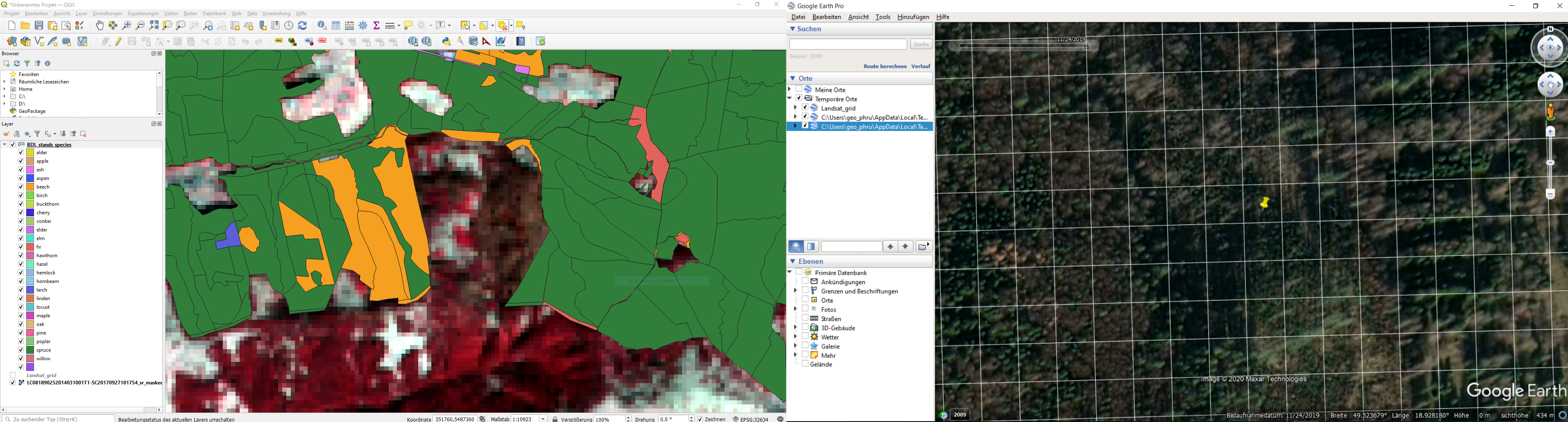
Exemplary setup of QGIS (left, includes forestry polygons, and Landsat images) and Google Earth (right, includes Landsat pixel grid as kml file, and historic images acquired during autumn), both linked with the Send2GE plugin
3) Explore your training data
- Explore the spectral-temporal behaviour of the different classes.
Load your shapefil/gpkg in R using readOGR(). Extract
the spectral values of the (1) NDVI, (2) TCB, (3) TCG and (4) TCW at
your point locations in R using the extract() function.
Specify sp = TRUE to append the spectral values to the
point shapefile.
To identify the spectral-temporal behaviour of the land cover classes, create visualizations of the surface reflectance values in your training data, grouped or colored according to the land cover class. For example:
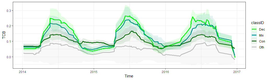
Spectral-temporal trajectory of the Tasseled Cap Brightness for the four different land cover classes
The R-code below shows how to extract the data, manipulate the dataframes and visualize the spectral-temporal profiles. Make sure you understand each step and feel free to adjust to your needs or desired output.
# =============================================================================
# load required packages (and install if necessary)
l_packages <- c("ggplot2", "Rcpp", "terra", "tidyverse", "zoo", "lubridate")

for (p in l_packages){
  if(! p %in% installed.packages()){
    install.packages(p, dependencies = TRUE)
  }
  library(p, character.only = T)
}

# =============================================================================
# 3) Explore your training data

# set working directory
dir_main <- ".../session_03-06"
setwd(dir_main)

# read time series of selected spectral bands | indices | transformations
tcb   <- rast("imagery/time-series/2014-2016_001-365_HL_TSA_LNDLG_TCB_TSS.tif")
tcg   <- rast("imagery/time-series/2014-2016_001-365_HL_TSA_LNDLG_TCG_TSS.tif")
tcw   <- rast("imagery/time-series/2014-2016_001-365_HL_TSA_LNDLG_TCW_TSS.tif")
ndvi  <- rast("imagery/time-series/2014-2016_001-365_HL_TSA_LNDLG_NDV_TSS.tif")
evi   <- rast("imagery/time-series/2014-2016_001-365_HL_TSA_LNDLG_EVI_TSS.tif")

# read training point locations
file_training_points <- "vector/s03_training_data.gpkg"
train <- vect(file_training_points)

# put imagery in list to extract points iteratively
l_imgs <- list(ndvi, evi, tcb, tcg, tcw)

# extract time series at training locations for each img in list
l_values <- lapply(l_imgs, FUN = terra::extract, train, method = 'simple',
                   bind = TRUE, xy = TRUE, ID = TRUE)

# convert (SpatialPoints)objects to dataframes
l_df <- lapply(l_values, as.data.frame)

# add name of spectral feature to associated dataframe
index_name <- c("NDVI", "EVI", "TCG", "TCB", "TCW")
for (i in 1:length(index_name)){
  l_df[[i]]$feature <- index_name[i]
}

# get column names that are not the time series values
not_timeseries <- names(l_df[[1]])[!grepl("20*" , names(l_df[[1]]))]

# prepare DFs with helper function
prep <- function(x){
  return(
    x %>%
      gather(time, value, -not_timeseries) %>%
      mutate(classID = factor(classID),
             time = as.Date(substr(time, 1, 8), format = "%Y%m%d"),
             value = value/10000)
  )
}

l_df <- lapply(l_df, prep)  # apply helper function to each df

# merge dfs into one df (long format)
df <- do.call(rbind, l_df)

# retrieve averages for each feature and class over time
df_mean <- df %>%
  group_by(feature, classID, time) %>%  # group to calculate for each separately
  summarise(mn = mean(value, na.rm = TRUE),
            sd = sd(value, na.rm = TRUE)) %>%  # get temporal mean and std
  mutate(roll_mn = rollapply(
    mn, width=6, FUN=function(x) mean(x, na.rm=TRUE), by=1, partial=TRUE,
    fill=NA, align="center"
  ),
  roll_sd = rollapply(
    sd, width=6, FUN=function(x) mean(x, na.rm=TRUE), by=1, partial=TRUE,
    fill=NA, align="center"))  # apply rolling mean to "smooth" trajectories


# =============================================================================
# 2) Visualize

# specify colours
colours <- c("green", "red", "blue", "grey")
scale_custom <- list(
  scale_color_manual(values = colours),
  scale_fill_manual(values = colours)
)

# plot e.g. mean TCW (+-1sd) over time for each class
feat <- "TCB"
ggplot(data = df_mean %>% filter(feature == feat)) +
  geom_line(aes(x=time, y=roll_mn, color=classID), size=1.25) +
  geom_ribbon(aes(x=time, ymin = roll_mn - roll_sd,
                  ymax = roll_mn + roll_sd, fill=classID), alpha=0.1) +
  scale_custom +
  labs(x ="Time", y = feat) +
  theme_bw()

# add month column
df_monthly <- df %>%
  group_by(feature, classID, time) %>%
  mutate(month = format(time, "%m"))
# visualize monthly distributions irrespective of year

feat <- "NDVI"
ggplot(data = df_monthly %>% filter(feature == feat)) +
  geom_boxplot(aes(x=as.factor(month), y=value, fill=classID)) +
  scale_custom +
  labs(x ="Time", y = feat) +
  theme_bw()
Based on your plots, try to answer the following questions:
- Does the NDVI/EVI and the Tasseled Cap components allow for discriminating the target classes?
- Which classes are likely difficult to separate?
- What is the advantage of multitemporal versus bi- and unitemporal imagery?
Reading materials
In the next session, we would like to discuss the following papers:
In this paper, a novel algorithm for large-area mapping was developed. Please read the paper thoroughly, make sure you understand the underlying concept and note questions of understanding or for general discussion. Please be guided by the following broader questions:
- What is the motivation of developing the described method?
- Which key parameters are considered for the parametric scoring?
- What is the difference between annual and seasonal consistency?
In this paper, the authors explored the concept of spectral-temporal metrics (STMs) for separating spectrally similar land cover classes in the Brazilian Cerrado. Please read the paper and make sure you understand the underlying concept. Write down questions of understanding and issues to discuss during the next session. Also, try to answer the following questions:
- How do STMs conceptually differ from pixel-based composites?
- For which type of (classification) problems could spectral-temporal metrics be useful?
Copyright © 2020 Humboldt-Universität zu Berlin. Department of Geography.
![]()