Raster data (in R)
Learning goals
- Recap ‘What is a raster?’ and the ‘remote sensing resolutions’
- Reading and writing of raster and vector data in R
- Resampling and (re-)projecting.
 Why code?
Why work with geospatial data, or any data really, in a programming environment and not only stick with Graphical User Interfaces (GUIs) like QGIS? For us it is particularily the flexibility of processing data and not being restricted to predetermined tools and functions. Also we often find ourselves having to apply a certain chain of processes repeatedly over different data. It is particularily the reusability of code that outcompetes working in a GUI in terms of efficiency. Last, getting acquainted with any programming language is generally a great and much in demand skill.
Help with coding
Once you enter the world of programming and you will come across syntax errors or tasks in which you need help with writing code. You are learning new a language after all. Good news is there are many excellent tutorials and community feedback out there which will help you tremendously in achieving your tasks. One great resource is the Stack Overflow community where people can ask code related questions and seek help from fellow (advanced) programmers. Make sure to Google your problem and chances are very high you come across a forum entry precisely matching your needs. Then, of course, there is ChatGPT. Last, do not unterestimate your own problem solving skills which will grow quickly in terms of coding with time spent doing so.
Background
Based on the content presented under the R basics and
Precourse subpages you are already equipped with a good
baseline for operating R in general and dealing with raster
data using terra in particular. In today´s session we will
built upon some of the workflows of the Precourse session, so
please navigate there and take another look if something is unclear at
first. Of course - as always - please do not hesitate to ask us in
person during the seminar or digitally using the Forum in
Moodle.
Now before we start our practicals for today, let`s draw a little outline on what we would like to do in the coming first sessions. One major goal of this course is to equip you with the tools to derive interpretable, meaningful information from remotely sensed imagery, which - among other goals - could be used for global change analyses. This information extraction process often encompasses using statistical or machine learning models to regress or classify the input spectral information into thematic or biophysical information. Most commonly this involves land cover mapping, e.g. for highly detailed information on European Land Cover or various crop types in Germany, only made possible across such large scales via remote sensing. Our first thematic goal for this course will be classifying tree or forest types for a region of the Carpathian Mountains.
In order to arrive at such land cover information, we generally need a good process understanding of our research target and must know how to (pre-)process and analyse the ‘raw’ remotely sensed imagery prior to making use of any model. Therefore, before we take a look at machine learning models in Session 5, we will first learn to get our data into shape. Specifically, the next four sessions will deal with …
- … the fundamentals of raster (and vector) data handling (today)
- … sensor calibration, atmospheric correction and data quality (particularily cloud masking)
- … spectral surface properties (focus on vegetation) and training data collection
- … image feature creation (best-available-pixel composites and spectra-temporal-metrics)
Remote sensing resolutions
Recall that remote sensing sensor systems can be broadly characterised along four resolutions:
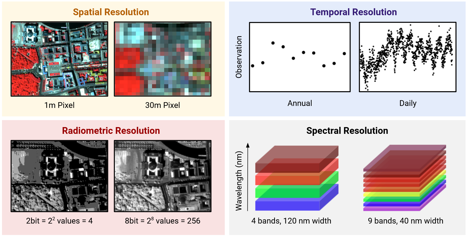
The four Remote Sensing resolutions that define the image data.
- The spatial resolution describes the length of one side of a single image pixel. Often, the term ground sample distance (GSD) is used interchangeably, which describes the distance between two adjacent pixel centers measured on the ground.
- The temporal resolution is the interval between two observations of the same spot on Earth. Note: There is a trade-off between spatial and temporal resolution as such that finer spatial resolution leads to lower observation density
- The radiometric resolution describes the range and discernible number of discrete gray values a sensor can distinguish. The radiometric resolution is measured in bit (binary digit). The radiometric resolution governs the datatype that needs to be used (we take a closer look at this in the next session)
- With spectral resolution we often refer to the width and number of spectral bands in the sensor system. Technically, it refers to the width of the wavelength interval of individual bands.
Unique sensor resolutions may then directly result in specific image properties of the raster data. For instance, the ‘OLI’ sensor onboard the Landsat-8 satellite measures large parts of the electromagnetic spectrum with a GSD of 30 meters. Accordingly, the default pixel width and height of the projected raster data is 30 meters.
Raster images
A quick warm-up of your GIS knowledge. The two most popular spatial data formats are vector and raster data. Digital images - including remote sensing imagery - are stored in rasters.
What is raster
data?A raster is a matrix of cells (pixels) organized into rows and columns.
You are familiar with common image formats such as .jpg
or .png. Generally, there are hundreds of different
image formats (see gdal.org), most common image
formats regarding digital remote sensing imagery are illustrated in the
table below:
| Format name | Extension | Description |
|---|---|---|
| GeoTIFF | .tif, .tiff, .gtiff | TIFF + geospatial reference |
| ENVI | generic, often used in imaging spectroscopy community; Header file (.hdr) with meta data! | |
| JPEG2000 | .jp2, .j2k | used by many data providers; usually for integer values only |
| HDF4, HDF5 | .hdf, .h4, .hdf4, .h5, .hdf5 | hierarchical data format, version 4 or 5; multi-resolution raster |
| netCDF | Network Common Data Format; multi-resolution raster | |
| SAVE | Standard Archive Format for Europe e.g. Sentinel-1 and Sentinel-2 |
The by far most common format used is the geospatial Tagged Image
File Format or GeoTIFF. What is important for data
formats when dealing with geospatial raster data is the ability to store
spatial metadata and (usually) to save the data lossless to disc,
i.e. the original recorded data is not manipulated or lost due to heavy
compression (e.g. .jpg is therefore not a suitable format
for remotely sensed data).
The raster data iself exhibits certain image properties:
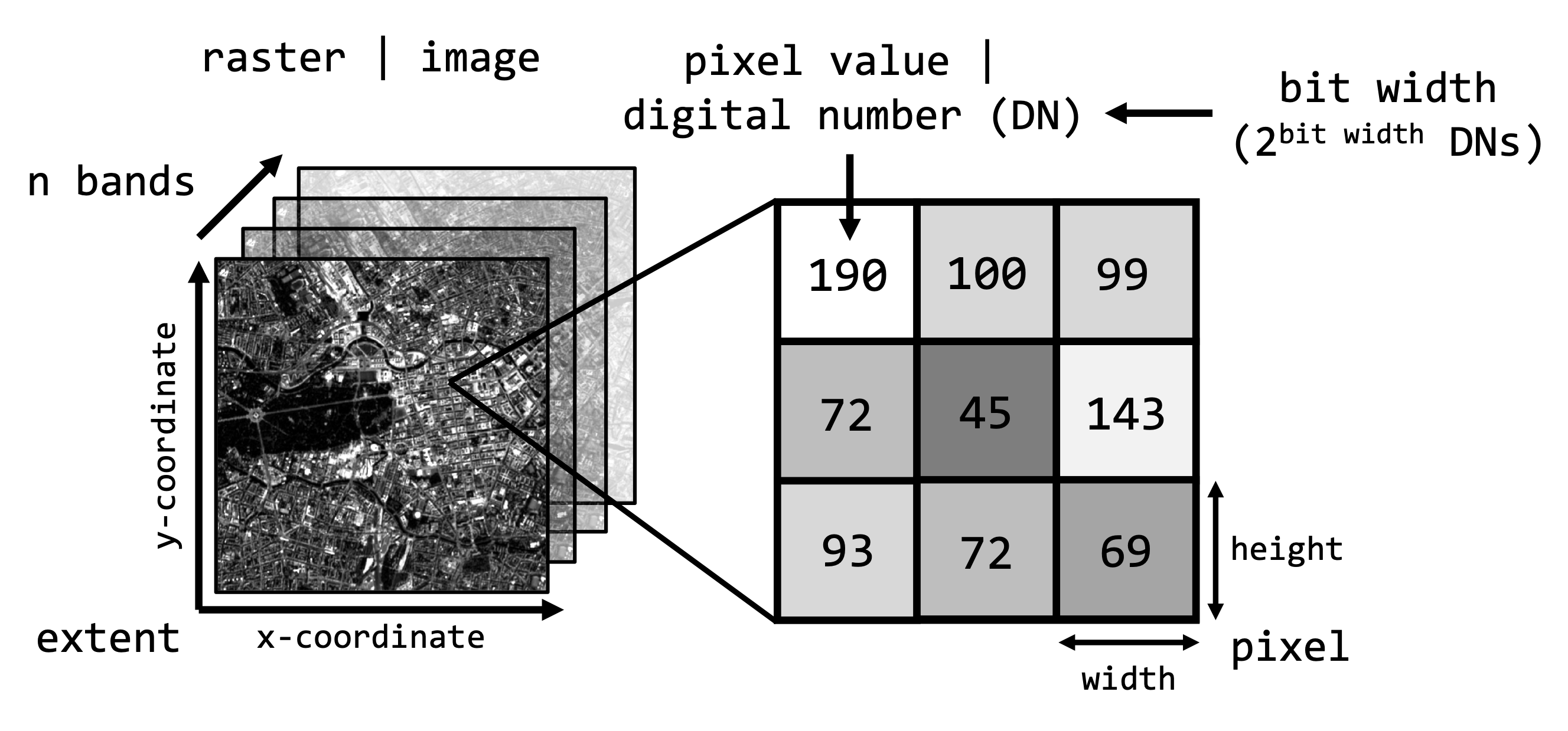
Below you find some terra-functions to access some of
these properties and particularily how to access individual bands or
pixels inside an image:
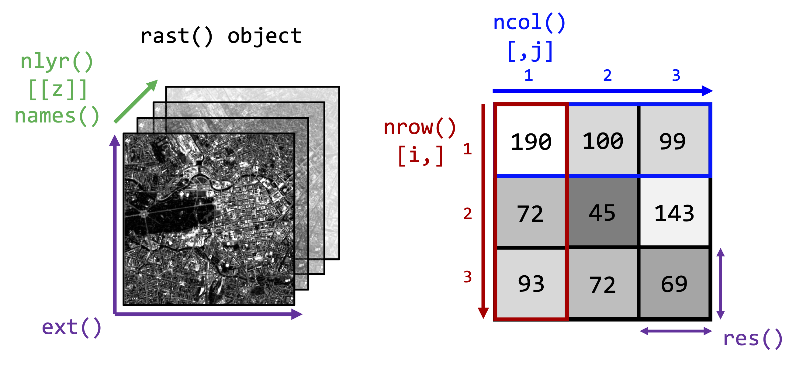
As you can see from the above figure, you can imagine the image as a
three-dimensional array in which each pixel has a xyz-coordinate or
index which we can access using square brackets [] on our
raster object.
Practicals
Data
For classifying tree types in the Carpathians we will make use of Landsat data. During the Precourse you learned how to access the data free of charge via the USGS Earth Explorer. For the remainder of the seminar we will provide you with the needed data (see Course data), which will be especially usefull when we not only look at one or two images but at image time series covering multiple years.
Take a look at the content of today´s and
next week´s session materials. The folder imagery
contains three Landsat-8 scene folders …
LC08_L1TP_189025_20140310_20200911_02_T1LC08_L1TP_189025_20140716_20200911_02_T1LC08_L2SP_189025_20140716_20200911_02_T1
… and a single-band file named reference.tif, which
defines the extent of our study area for the forest type analysis.
The folder vector contains the GeoPackage-file
BDL_stand-species.gpkg which is forestry data collected in
2015 (publicly available here). We have
prepared this vector file to contain - among other attributes - the
following:
| Attribute field | Definition | Class |
|---|---|---|
| species_en | Dominant genus in each stand | Ash, Beech, Fir, Spruce… |
| part_cd | Share of this genus within the stand | 0 – 100 (in %) |
Today we will only need the single Landsat scene
LC08_L1TP_189025_20140310_20200911_02_T1, thus the scene
acquired on March 10th 2014. Furthermore, we are going to need
reference.tif and BDL_stand-species.gpkg.
Let´s take a look at the datasets in R. For this we start with importing the needed libraries and setting our working directory:
# load required packages (and install if necessary)
l_packages <- c("terra") # you can put all needed libraries in the future here; today we only need the "terra" package
for (p in l_packages){  # for-loop iterates over items in "l_packages" vector
  if(! p %in% installed.packages()){  # if the item, i.e. package is not installed, then install
    install.packages(p, dependencies = TRUE)
  }
  library(p, character.only = T)  # load required package
}

# set working directory
setwd(".../eo_data_s01-02")
We will start of with the Landsat data. The goal is to read in the single bands we need, create a multiband stack, and write the result to disc.
Exercise 1
Read the blue, green, red, near-infrared
(nir), shortwave-infrared 1 (sw1), and shortwave-infrared 2
(sw2) bands of the Landsat scene acquired on the 10th of March into
a multiband raster stack.
You can identify the correct image from the Landsat file naming convention, and the needed band-files by checking the list of Landsat spectral bands and/or the following figure:
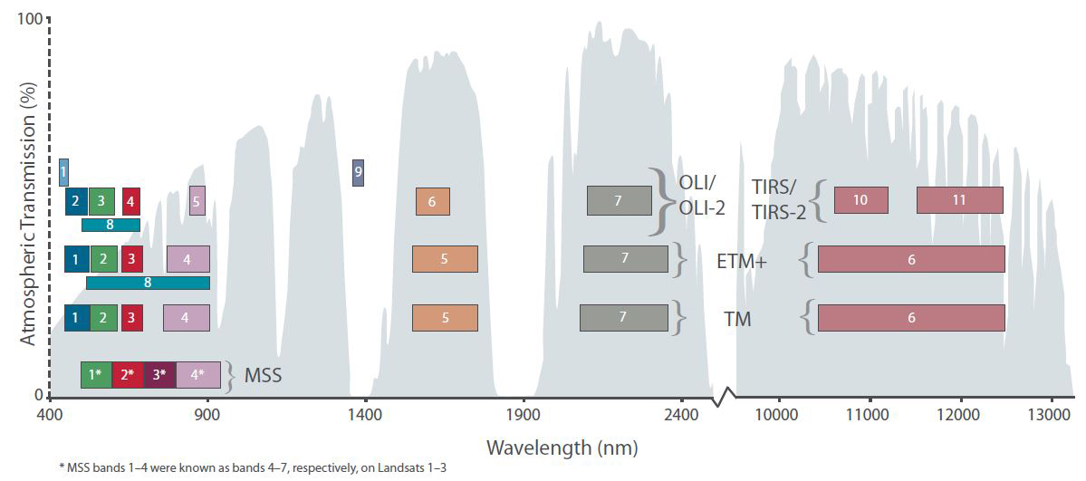
Band designations for the Landsat satellites
Once you know which files to include, create a list using the
list.files() function, create a raster stack using
rast(), rename the bands (e.g.
c("BLU", "GRN", "RED", "NIR", "SW1", "SW2")). Remember to
use ?list.files to seek help for correct function usage,
specifically for the arguments pattern and
full.names.
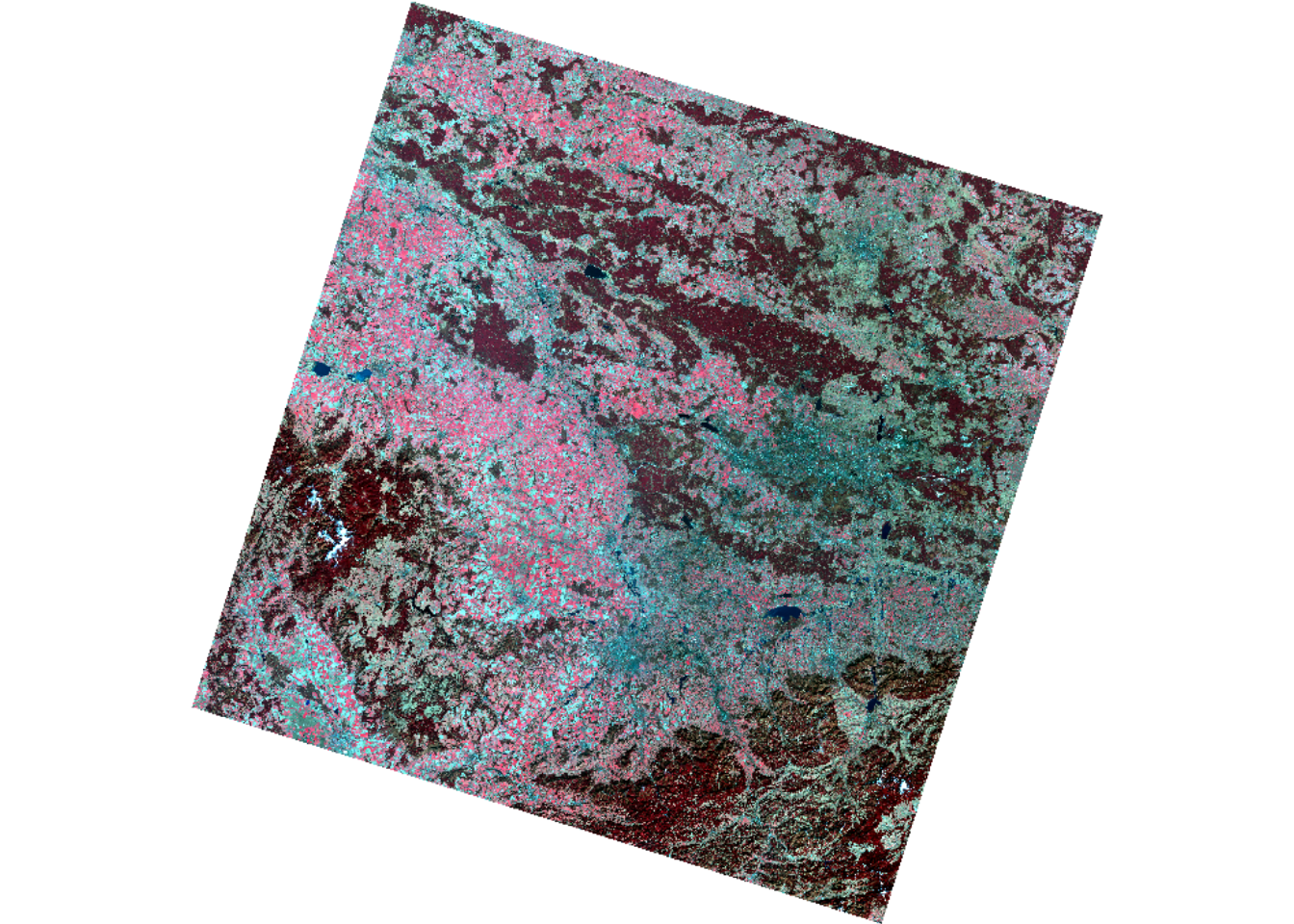
Use the plotRGB-function to visualize the data as
false-colour representation showing vital vegetation in red colours. Use
help(plotRGB) or ?plotRGB to learn how to use
this function, i.e. the arguments of the function. Hint: you
need 5 arguments of the function and the index, i.e. the
position of each band along the z-dimension of the image. Below you find
the desired visual result.
Take a look at the value range of the single Landsat bands. If you
remember, the Landsat data is delivered in Digital Numbers
(DNs), i.e. if we would like to have interpretable values in
the form of Reflectance [%], we must first scale the
DNs using the sensor-specific calibration coefficients found in the
metadata
(LC08_L1TP_189025_20140310_20200911_02_T1_MTL.txt). In the
next session we will unravel why this step is important. For now, in
order to scale your multiband raster from DNs to reflectance, simply
apply the following equation to your raster object:
\[Reflectance = 0.00002 * DN - 0.1\]
Scale your multiband raster from DNs to reflectance using the above linear equation. Verify your result and save the resulting multiband raster to disc. Open the raster stack in QGIS and experiment with the visualization settings to create a falce-colour visualization just as above.
# plot
plot(img_march)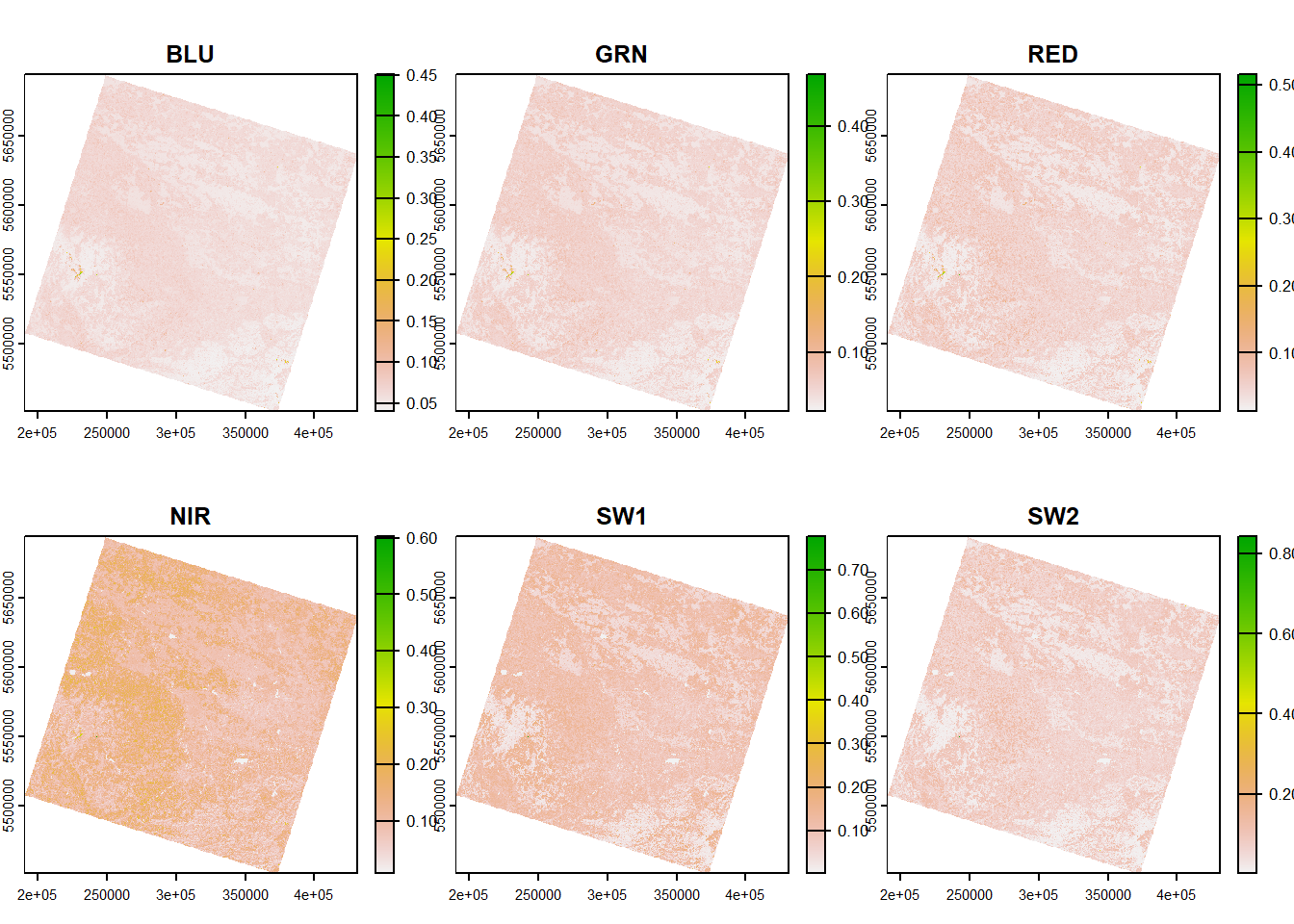
As you can see from the plot, the range is now between 0 and 1, representing the percentage reflected and measured by the sensor.
Vector
Second, we will now take a look at the vector data.
Read the vector dataset (
BDL_stand-species.gpkg) also into QGIS and take a look at
the attribute table. Next, read in the vector dataset into R using
terra´s vect()-function. Again, take a look at
the attribute table (data.frame) and plot the
data.
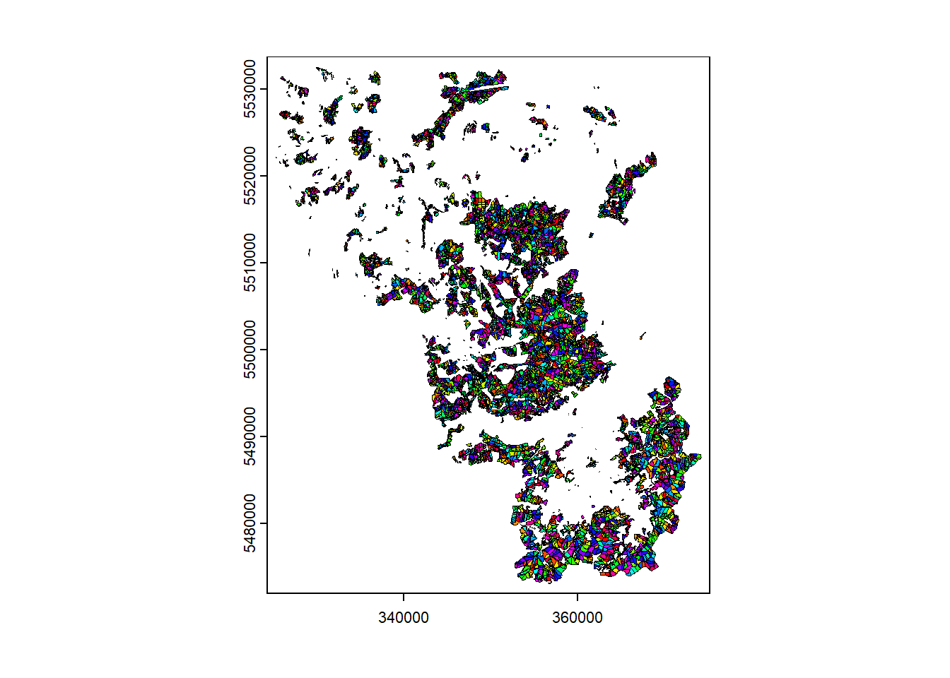
As you can see the forest data are polygons for which a variety of attributes are available:
| Attribute field | Definition | Class |
|---|---|---|
| species_en | Dominant genus in each stand | Ash, Beech, Fir, Spruce… |
| part_cd | Share of this genus within the stand | 0 – 100 (in %) |
We are interested in species_en and
part_cd. species_en describes the dominant
genus in each stand and part_cd provides the associated
percentage this genus contributes overall.
Identify how many unique genera of trees are recorded in the dataset?
Although the information on the genera will be valuable later on,
what we would like to have now, is a simplification of the genera into
the leaf phenology types evergreen and
deciduous. We can manipulate the SpatVect like a
data.frame or convert the attributes into a
data.frame and continue from there.
Exercise 5
Complement the vector dataset by an additional
attribute type which holds 1 for deciduous
genera and 3 for evergreen genera. Below you find the first
steps and a description of what each step does. Try to fill in the code
for the last two steps (or come up with an entirely different way). If
you are stuck, exchange with others and only if you are close to
despair, find the solution below.
# convert SpatVect object into data.frame
df_forest <- as.data.frame(vec_forest)

# identify unique genera and sort alphabetically
genera_sorted <- sort(unique(df_forest$species_en))
# print(genera_sorted)
# manually create vector for deciduous = 1 and evergeen = 3 according to "print(genera_sorted)"
v_type <- c(1,1,1,1,1,1,1,1,1,1,1,3,1,1,3,1,1,1,1,1,1,3,1,3,1)
# create look-up table
df_lookup <- as.data.frame(cbind(genera_sorted, v_type))

# create new column/attribute in data.frame and add values by matching "species_en" to "df_lookup"

# add column to SpatVect
Click here only if you are stuck
# create new column/attribute in data.frame and add values by matching "species_en" to "df_lookup"
df_forest["type"] <- as.numeric(df_lookup$v_type[match(unlist(df_forest$species_en), df_lookup$genera_sorted)])
# add column to SpatVect
vec_forest <- cbind(vec_forest, df_forest["type"])
Note that if we do not really need to work on/with
data.frames, we can also directly manipulate on the
SpatVect object like so:
# identify unique genera and sort alphabetically
genera_sorted <- sort(unique(vec_forest$species_en))
# manually create vector for deciduous = 1 and evergeen = 3 according to "print(genera_sorted)"
v_type <- c(1,1,1,1,1,1,1,1,1,1,1,3,1,1,3,1,1,1,1,1,1,3,1,3,1)
df_lookup <- as.data.frame(cbind(genera_sorted, v_type))
# create new column/attribute and add values by matching "species_en" to "df_lookup"
vec_forest[["type"]] <- as.numeric(df_lookup$v_type[match(unlist(vec_forest$species_en), df_lookup$genera_sorted)])
Vector to Raster (“Rasterization”)
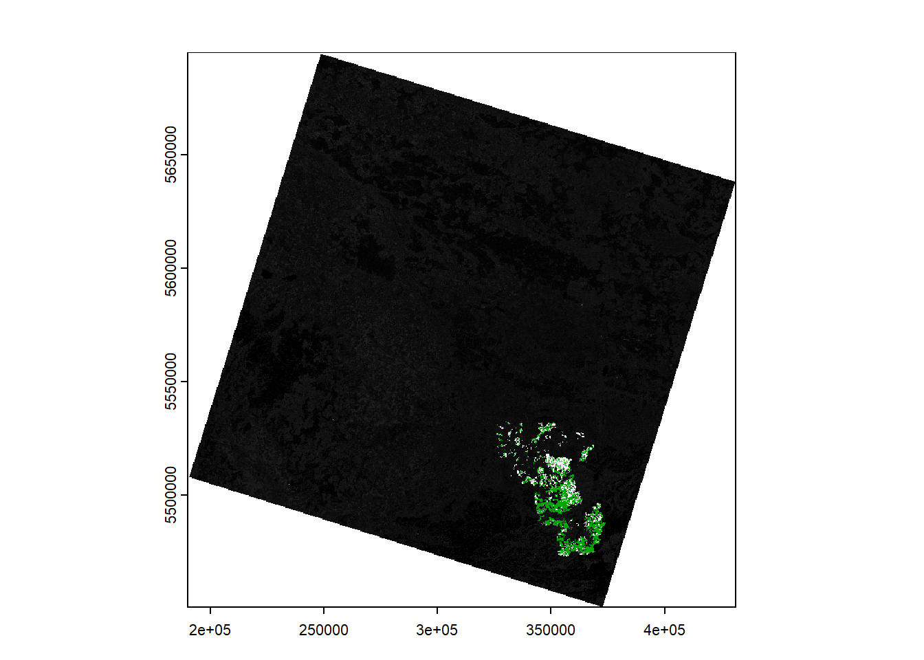
Now that we have the information from the vector data and the raster bands loaded into a multiband image, we want to rasterize our newly created attribute to match the Landsat data. This will allow to subset our data later on when we take a closer look at the forest types.
Rasterize the new
type attribute of
the vector dataset using rasterize. Plot your result to
make sure the 1s and 3s are correctly ‘burned’
into the raster.
Reprojecting - Resampling - Interpolating
Last for today, we want to spatially subset our data to the extent we
are actually interested in. Our study area extent and the data from
Session 3 onwards are defined by
reference.tif.
Compare the Coordinate Reference Systems (CRS) / projections of the three datasets (Landsat image, rasterized vector, and reference).
When you compare the Coordinate Reference Systems
(CRS) you will notice that we must reproject the Landsat and
vector data to match reference.tif. The following figure
depicts a zoom-in comparing the 30x30m grid of
reference.tif shown in red (EPSG:3035), to the
30x30m grid of
LC08_L1TP_189025_20140310_20200911_02_T1_B5.tif beneath
(EPSG:32634).
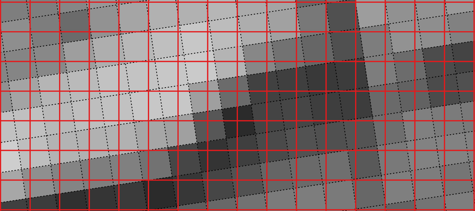
Mismatch in raster grids between two CRSs
If we reproject
LC08_L1TP_189025_20140310_20200911_02_T1_B5.tif now onto
the grid defined by reference.tif, we must choose a
resampling method which defines the way the values in
the output raster will be computed from the input raster. The three most
commonly used techniques are Nearest Neighbour, Bilinear
Interpolation and Cubic Convolution:
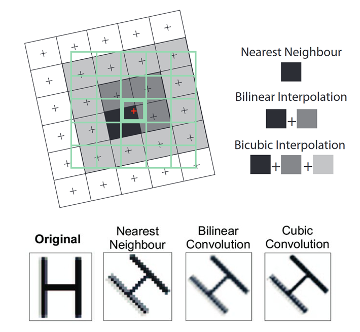
Three common resampling methods - Source: “Principles of Remote Sensing” © 2009 by ITC, Enschede
- Nearest Neighbour: The value of each cell in an output raster is calculated using the value of the nearest cell in an input raster.
- Bilinear Interpolation: The value of each cell in an output raster is calculated using the weighted average value of the nearest four cells in an input raster.
- Cubic Convolution: The value of each cell in an output raster is calculated using the weighted average value of the nearest 16 cells in an input raster.
To reproject your data in R you can make use of the
project function of the terra package.
Exercise 8
Take a closer look at the arguments of the
project function.
First, our goal will be to project the Landsat multiband raster as
well as your rasterized forest-type dataset into the extent and CRS of
reference.tif. Discuss on the needed resampling methods and
necessary arguments to achieve this goal. Why should you ideally choose
different resampling algorithms for this task?
Then, also reproject the forest vector dataset using
project.
writeRaster and writeVector. Choose
appropriate filenames and in preparation for next week you may look into
which datatype for the raster datasets are suitable.
Reading materials
In the next session, we would like to discuss the following paper:
This is a rather technical reading, which introduces the Fmask algorithm for automated cloud and cloud shadow detection. It has been widely used for cloud detection on Landsat TM and ETM+ data, and was enhanced for the use with Landsat OLI and Sentinel 2 data (documented in Zhu et al. 2015 and Qiu et al. 2019).
While reading focus on the following questions:
- Why do we need automated cloud masking?
- Where are the limitations?
- How will different error types impact further analyses? Do you consider omission or comission errors to be more severe?
Copyright © 2020 Humboldt-Universität zu Berlin. Department of Geography.
![]()