6. Data acquisition and multi-temporal imagery
Learning goals
- Accessing and downloading freely available multispectral data by …
- … getting to know ESA’s Copernicus Open Access Hub and USGS’ EarthExplorer, and …
- … searching for Sentinel-2 and Landsat data.
- Identifying the intra-annual spectral-temporal behaviour of land
cover in Berlin, …
- … by creating a time-series image stack of 2019 Sentinel-2 imagery.
Sentinel-2 and Landsat
The European Union’s Copernicus program features several Earth observing satellites, including a pair of satellites carrying high resolution optical sensors: Sentinel-2A (S2A) and Sentinel-2B (S2B). The satellites were launched recently, S2A in June 2015, S2B in March 2017. The sensor on board is called Multispectral Imager (MSI). Each satellite overpasses the same place on Earth every ten days. Combined, both satellites yield a revisit time of 5 days, recording with 290 km swath width.
The Landsat mission comprises eight multispectral Earth observing satellites, with Landsat-1 initially launched in 1972. From the launches of Landsat-4 and Landsat-5 Thematic Mapper’s (TM) onwards, the Landsat mission featured at least six key bands in the optical domain at 30m spatial resolution: blue, green, red, nIR, SWIR1 and SWIR2.
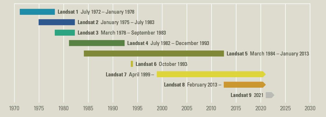
The Landsat mission timeline (Source: USGS)
The Sentinel-2 MSI has 13 spectral bands, which partly resemble the Landsat spectral bands but also add new spectral regions, such as the red edge bands. The bands have varying spatial resolutions of 10, 20, or 60 m. The three visible bands blue, green, red, and a broad nIR band come at 10 m spatial resolution (bands 2, 3, 4, and 8). Red edge bands, a narrow nIR band, and the swIR bands come at 20 m spatial resolution (bands 5, 6, 7, 8a, 11, and 12).
The Landsat sensor family has a swadth width of ~185 km, a 16-day repeat cycle by one sensor (i.e., 8-day repeat cycle by two sensors), which new missions such as the Sentinel-2 family outperform. However, the continuous long-term archive of 30m Landsat imagery is truly unique and allows for multi-decadal assessments of land surface change on Earth.
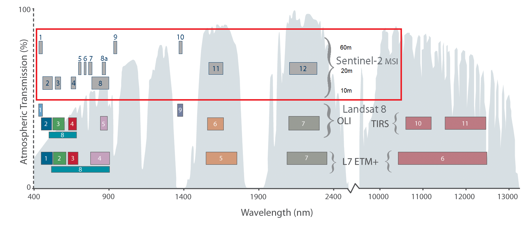
Comparison of Sentinel 2 with Landsat 7 and 8 spectral bands (Source: USGS).
Data providers
Image archives such as the Sentinel-2, Landsat or MODIS data catalog represent enormous data volumes, growing larger every day. Who stores the data and how is it made accessible to users?
Public institutions such as the the European Space Agency (ESA) and the United States Geological Survey (USGS) play a key role in this regard, as they host the currently most relevant platforms for Earth Observation data distribution - the Copernicus Open Access Hub and the USGS Earth Explorer. Most (but not all) of the data provided on these platforms are currently available free of charge.
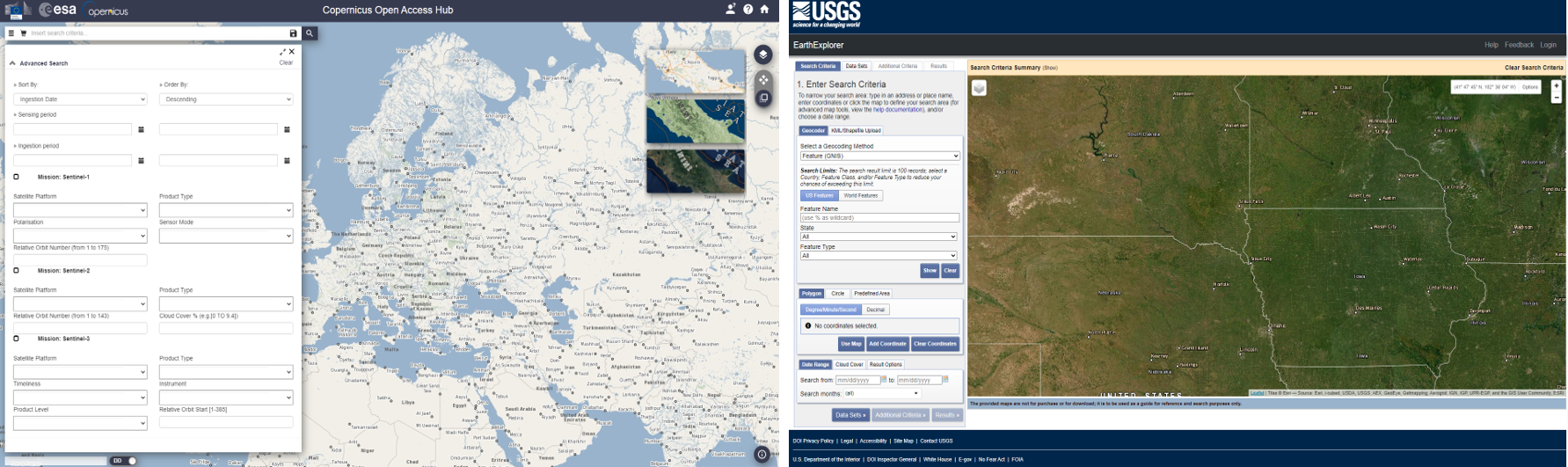
Copernicus Open Access Hub and USGS Earth Explorer.
-
Zoom to Berlin and then switch to Area Mode:

- Draw a region-of-interest (ROI) to approx. cover the greater Berlin study area from the previous sessions.
-
Open the search bar
 and filter using the following criteria:
- Mission: Sentinel-2
- Product Type: S2MSI2A
- Sensing period: 2019/01/01 to 2019/12/31
-
First save
 ,
then start
,
then start  the
search
the
search
- What are the available product types - specifically: How do S2MSI1C and S2MSI2A differ?
- What determines the spatial footprint of the displayed imagery (i.e. rectangles, overlaps, trapezoid-like shapes)?
- How many images are available for the T33UUU-granule in 2019?
-
Adjust the settings to only include images with
<= 10% cloud cover. How many images are left? - How does the number of scenes compare to available Sentinel-2 data?
- Why could setting a conservative cloud threshold be more restrictive
and unsuitable compared to Sentinel-2? To answer this, you may want to
remove the cloud cover threshold and then take a look at the preview
images by clicking
 for
a selected Landsat scene.
for
a selected Landsat scene.
Sentinel-2 data
Visit the Copernicus Open Access Hub and login or create a user account if you have not registered yet.
Once you are logged-in:You can fine-tune your search using pattern-matching,
i.e. search for specific occurences of characters in the filenames. To
do so, first make sure you saved a search, then load the search (user
profile settings) and edit the text-string that will appear in the
search bar according to your needs: Full text
search. For example, to only search for the specific image-granule
T33UUU, add AND(filename:*T33UUU*) to the search
string.
Landsat data
Accessing Landsat data works in a similar
fashion: Visit the USGS Earth
Explorer. To search for imagery, you will not need an account, only
for downloading the data. Repeat the search with the specified criteria
from above for Landsat-8 Collection 2 Level-2 data.
Multi-temporal imagery
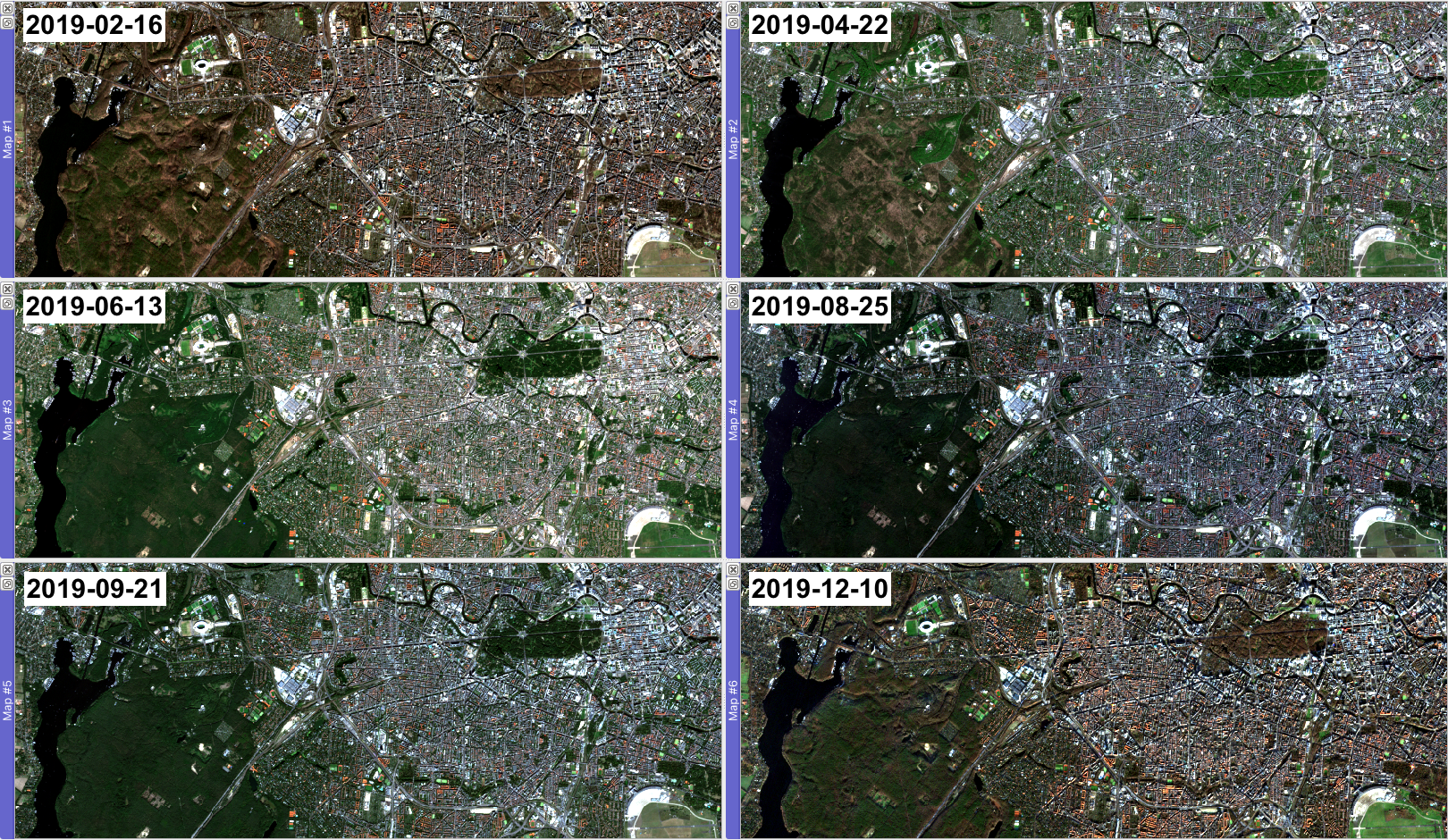
Based on your search from above, we have taken a further step and
ordered and downloaded Sentinel-2 L2A data for six additional time
steps: 2019-02-16, 2019-04-22,
2019-06-13, 2019-08-25,
2019-09-21, and 2019-12-10 - all of which you
can find in the Sentinel-2 data folder of the session
materials
(fe1_data_s05-09/Sentinel-2/S2A_L2A_T33UUU_2019XXXX_20m_9bands_berlin.tif):
Last week you explored the spectral signatures of the six land cover classes built-up, herbaceous, deciduous woody, evergreen woody, cropland and water in the Sentinel-2 image from the 26th of July 2019:
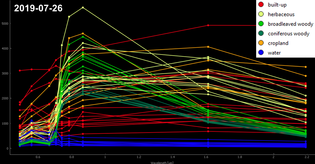
Today we are going to explore the intra-annual
spectral-temporal behaviour of our six land cover
classes. From the single date summer image (2019-07-26) we
could infer that some classes are clearly distinguishable, while others
appear fairly similar spectrally. We also know that these existing
ambiguities in our pure surface spectra are only going to increase with
increasing mixtures of the surfaces within single pixels
(mixed-pixel problem). In the laboratory we already examined
three phenological stages of deciduous woody vegetation. Now it is time
we incorporate the temporal dimension also into our image analyses.
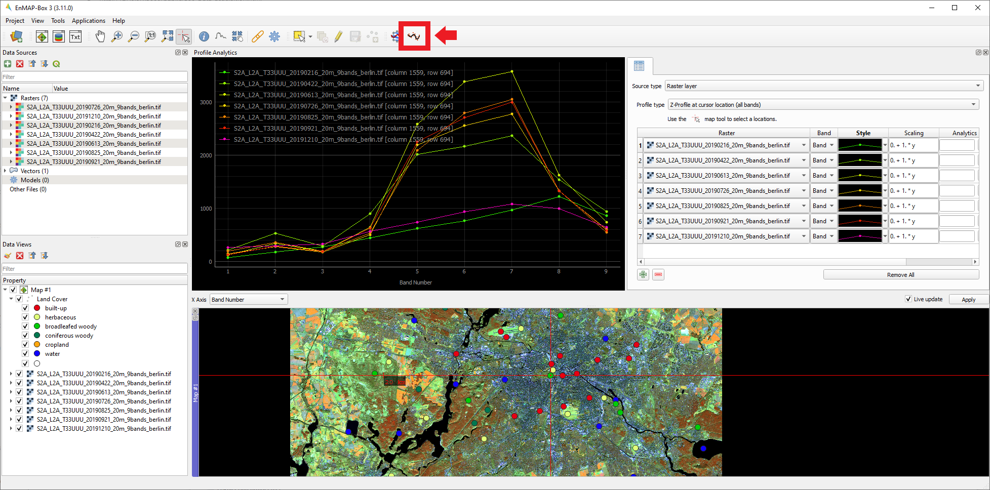
1) Visual exploration of spectral profiles
In a first step, …
Read the seven Sentinel-2 images into the EnMAP-Box and visualize the images in the false-color representation
R: SW1 | G: NIR | B: RED(tipp: once you adjusted the settings for one image, right-click onto the layer and selectCopy Style. On the other images you can usePaste Styleto directly adjust their band arrangement)Add your
.gpkgreference land cover points to the mapOpen the
Profile Analyticstool located at the
top bar and add
located at the
top bar and add  all
seven images to the visualization. Adjust the colors of each image
spectra to be able to differentiate between the acquisition
dates.
all
seven images to the visualization. Adjust the colors of each image
spectra to be able to differentiate between the acquisition
dates.Navigate to some of your sampled points and identify the spectral-profiles for the specific land cover types for the seven time steps:
-
From your selection of points, which of the classes’ spectra appear
rather similar over time, which rather different? Is the temporal
difference of the spectra equally pronounced for all bands?
2) Multi-temporal false-color image
The Profile Analytics tool points towards
spectral-temporal variation for selected class-band combinations. In a
next step, our goal will be to create a multi-temporal raster
stack which we can then visualize in false-color. This will
help us gain an understanding of the spectral-temporal behaviour across
our entire study area. Since the NIR band showed quite some
spectral variation over the course of the year for certain classes, we
will first create such a stack from the NIR band of each
Sentinel-2 image.
Open Applications > Raster Math (documentation)(=
the new version of the ImageMath Calculator):
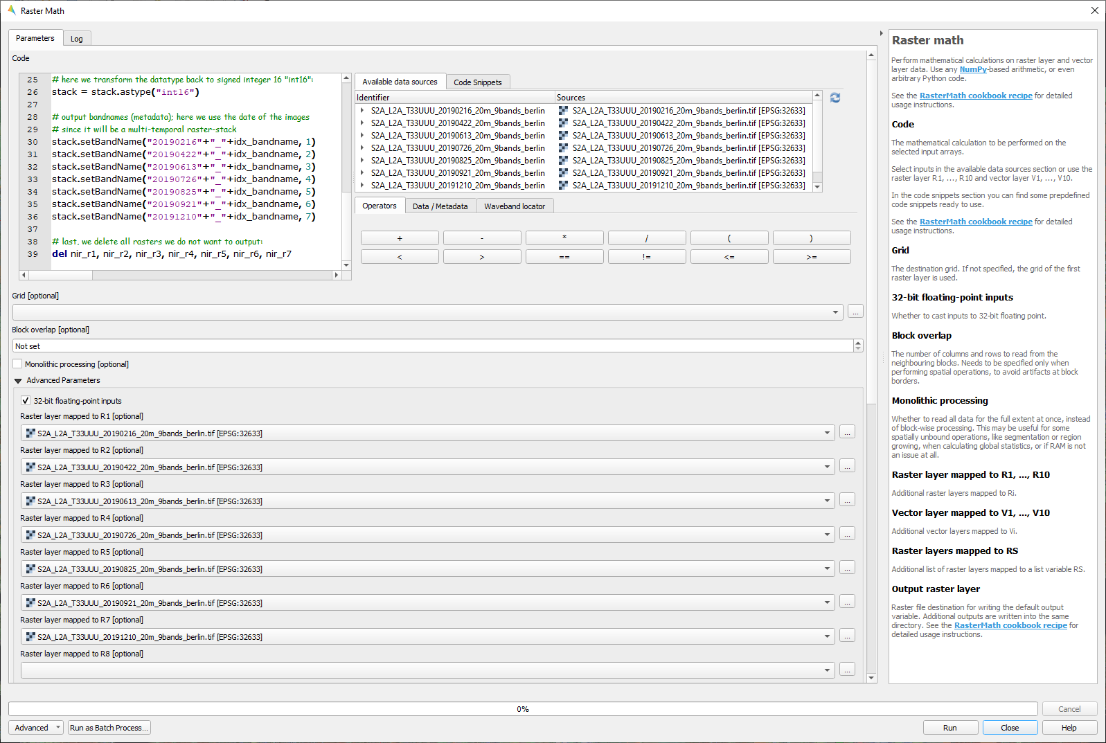
The main sections are the Code window on the left, the
Data Sources panel on the right, and the
Advanced Parameters section at the bottom. In the
Code window we can manipulate our variables using
Python syntax and Data Sources displays the
available image and vector files (= Sources) and automatically
assigns a variable based on their filename (= Identifier). The
Advanced Parameters section provides an easy way of
assigning raster and vector data sources to raster (R1,
R2, …) and vector (V1, V2, …)
variables to be used in the Code window.
The following code creates a multi-temporal raster stack from a specified band in our seven input images:
# define single band which we want to extract for each image
idx = 6  # index "6" refers to the 7th band since indexing starts at 0 (i.e., idx 0 = band 1)
idx_bandname = "NIR"  # this is the band at idx 6 and will be used as part of the  output bandname

# create an image stack from the single band
# here i.e. a multi-temporal image stack of the specified band (= "idx")
# note that R1, R2, ... R7 must be defined in the "Advanced parameters" section of "Raster Math"
stack = np.array(
    [R1[idx], R2[idx], R3[idx], R4[idx], R5[idx], R6[idx], R7[idx]]
)

# when the rasters are read into memory (R1, R2, ...) they are cast to float32;
# here we transform the datatype back to their original datatye, i.e. signed integer 16 or
# "int16" in numpy-syntax:
stack = stack.astype("int16")

# here we create a list "bandnames" which contains the dates of the single bands in out stack
bandnames = [
    "20190216", "20190422", "20190613",
    "20190726", "20190825","20190921",
    "20191210"
]
# to each date we add the spectral band name we selected above (here: "NIR")
bandnames = [b+"_"+idx_bandname for b in bandnames]
# the list looks now like this: ["20190216_NIR", "20190422_NIR", ..., "20191210_NIR"]

# last, we loop/iterate over each band in our 7-band raster stack
# it starts with the first band at index position 0 and loops until the last band
# at index position 6; each time it sets the correct name of the current band based
# on the "bandnames"-list we created
for b in range(len(stack)):
    stack.setBandName(bandnames[b], b+1)
Copy the code into the Code window and try to comprehend
the single steps with the help of the #-marked comments.
Before running the code, make sure (R1, R2, …,
R7) are defined in the Advanced Parameters in
the correct order (by date).
The output of this is a 7-band raster stack stack.tif
containing only the NIR band of each Sentinel-2 image. Open
the created image in the map view using the following false-color
representation:
R: 20190613_NIR | G: 20190726_NIR | B: 20190825_NIR:
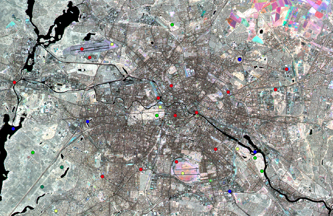
- What does the appearance of color mean for the general spectral-temporal behaviour - variation? - no variation?
- Which surfaces appear white-ish, which black-ish?
- Try out different false-color combinations and see if you can
identify specfic classes more easily compared to only using the
2019-07-26Sentinel-2 scene.
Assignment
We are moving closer to creating our first land cover map. Today you will complement your insights on the spectral behaviour of the classes by the temporal dimension. Thus, the goal of today’s assignment is to …
- … compare the spectral-temporal trajectories of the six land cover classes and thereby …
- … identify time-band combinations which allow for seperating the classes from one another.
For this you will make use of the reference points you sampled during
the last assignment as well as multi-temporal stacks (such as the
NIR-stack you created in above’s exercise).
In order to visualize the multi-temporal spectra for your sampled points:
- Make sure the NIR stack and your points are both loaded into a map view.
- Open the attribute table of your point dataset
(
Right-click > Open Attribute Table) and activate edit mode . Next, click delete field
 select and delete
(only!) the
select and delete
(only!) the Profilescolumn. Save edit and exit the attribute table. - Now open the
Spectral Librarytool and select
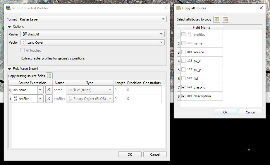
Import spectral profiles from other data sources in the tool window:
 - For
Formatselect Raster Layer, forRasteryour NIR-stack and forVectoryour reference points. ClickCopy missing source fields and select your
class-idanddescriptioncolumn:
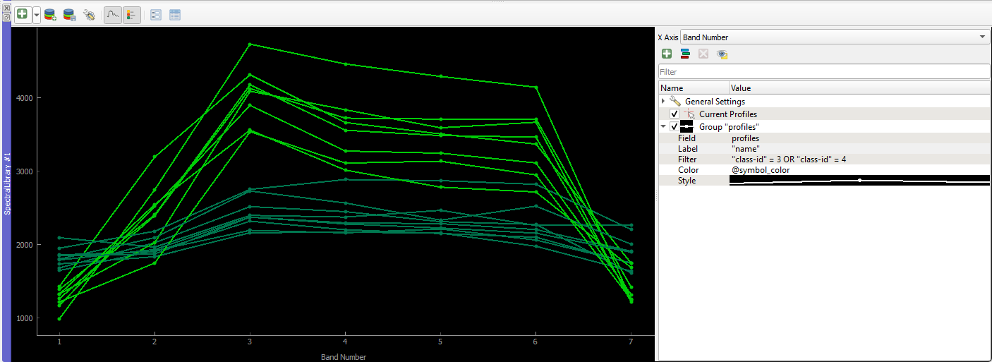
- Once the spectral-temporal profiles are imported, visualize them according to your land cover classes like in the previous session.
Your task is now to briefly describe the spectral-temporal trajectories of each class and to identify if certain classes can be differentiated from one and another. Please document your insights and the band-time combination for at least two pairs of classes.
Since the spaghetti-plot can be quite confusing, you can filter to
only show selected class(es) by opening the
Visualization Settings ![]() and using the
and using the Filter attribute under the
Group 'profiles' section. To filter for single classes,
paste "class-id" = 1 (for built-up) into the
Filter attribute, for multiple classes use the
OR-statement:
"class-id" = 3 OR "class-id" = 4:
Voluntary part: Repeat the above process by creating
a raster stack for the SWIR2 band.
Submission
Document your answers to the questions above with bullet points and the help of your screenshots in PowerPoint, Word or another software package.
Upload your answers/interpretations as
.pdffile.General submission notes: Submission deadline is the following Monday at 10am.
Copyright © 2023 Humboldt-Universität zu Berlin. Department of Geography.
![]()