10. Change Detection

Learning goals

Understand the principles of change detection
Conduct bi-temporal change detection of forest cover in the Brazilian Amazon

Change detection principles

Remote sensing provides great opportunities to observe and monitor changes on the land surface. Using satellite based images, changes over long periods of time as well as over large areas can be revealed. This section aims at providing insights into the most basic form of change detection - the bi-temporal change detection.

Bi-temporal change detection

To illustrate the procedure for bi-temporal change detection, we consider a hypothetical example of deforestation mapping. We would like to assess changes in forest cover, thereby revealing potential forest loss, gain, and stability.

We are given two images for the same study site, one from 1992 and one from 2011.

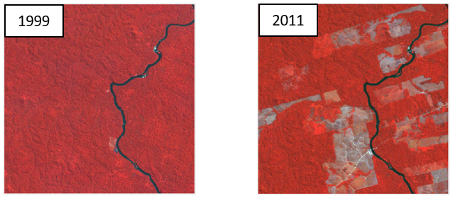
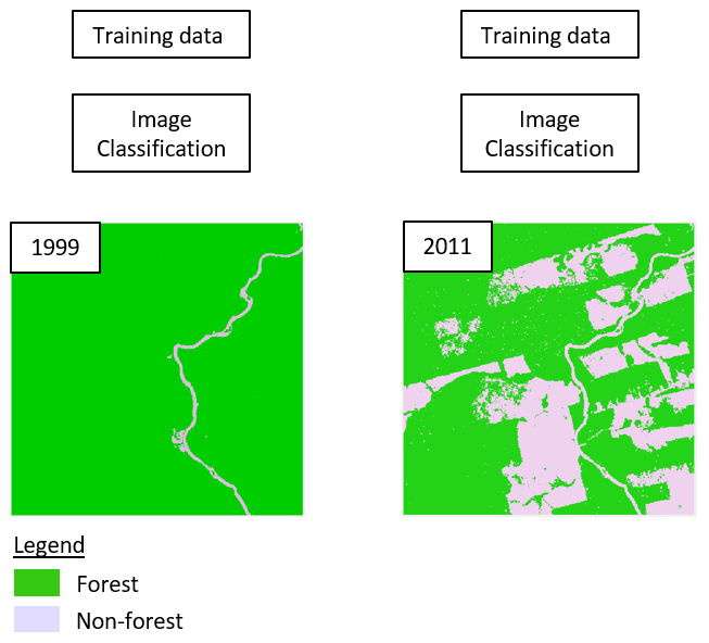
Landsat images for 1992 and 2011 in false-color visualization

For each image we want to produce a binary map showing forest / non-forest. To do so, we collect two sets of training data points: one for both classes in each image. Next, we use supervised classification techniques (e.g. Random Forest) to create one map per image. In this case we train one classification model for each image.

Creating binary classifications for 1992 and 2011

As a next step, we want to derive change information from the two maps. We can therefore combine the maps in order to assess class trajectories for each pixel. Remember, the classes in the map correspond to numeric values, e.g. 1 (forest) and 2 (non-forest). Since we observe bi-temporal change of a binary (2 classes) map, we can have \(classes^{timesteps} = 2^{2} = 4\) different sequences and thus change classes.

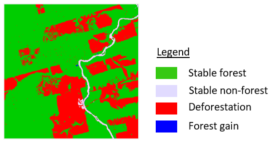
This map allows us to assess if change has occurred or not. In the binary case we can observe two types of stable sites

Stable forests: pixels with class label forest in 1992 and forest in 2011
Stable non-forests: pixels with class label non-forest in 1992 and non-forest in 2011

Also, we can observe two change classes

Deforestation: pixels with class label forest in 1992 and non-forest in 2011
Forest gain: pixels with class label non-forest in 1992 and forest in 2011

Or in tabular form:

Class 1992	Class 2011	Change class description	Change class ID
1	1	Stable Forest	11
2	2	Stable Non-Forest	22
1	2	Deforestation	12
2	1	Forest Gain	21

To create a third map that contains these four classes, we can use a simple mathematical trick: The most straightforward is to multiply the pixel values of the first image with 10 and then add the pixel values of the second image. As an example:

Stable forest (forest to forest): 1 * 10 + 1 = 11
Deforestation (forest to non-forest): 1 * 10 + 2 = 12

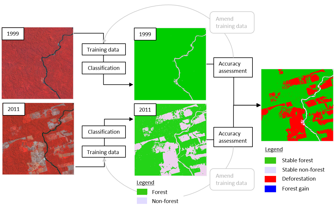
Change map showing all possible change classes

Overall Workflow

Let’s put this whole process of creating the maps and assessing change into a single workflow. It can be divided in six steps and summarized graphically as follows:

Bi-temporal change detection workflow

Exercise

Download the session materials from our shared repository.

The exercise for today deals with implementing this entire process chain, with a focus on the change detection (i.e. the classification process is already pre-coded and you only have to copy and comprehend the code).

The following datasets are available to you:

Training data training_brazil_forest.gpkg: “Forest” (classID: 1) and “Non-Forest” (classID: 2) reference points for both timesteps
Image features LT5_227065_19920808_subset.tif and LT5_227065_20110718_subset.tif: Two Landsat-5 images from 1992 and 2011

Land Cover Mapping

We will repeat the classification workflow from Session 8 and Session 9:

Data preparation: Extract the feature values of the Landsat-5 image at the training point locations into a data.frame
Model building: Supply the feature-label data.frame to the randomForest-function
Validation (internal model evaluation using Out-Of-Bag (OOB) error)
Prediction: Classify the Landsat-5 image using the image data, model, and the terra::predict function

The only difference being here that we have to build two models and also predict land cover twice. Here is the code to achieve this:

library(randomForest)

# input data
img_1992 <- rast()
img_2011 <- rast()
train_forest <- vect()


# rename bandnames
bandnames <- c("BLU", "GRN", "RED", "NIR", "SW1", "SW2")
names(img_1992) <- bandnames
names(img_2011) <- bandnames

# 1992
df_1992 <- data.frame(
  terra::extract(x=img_1992, y=train_forest["LC_1992"], bind=TRUE)
)
df_1992$LC_1992 <- as.factor(df_1992$LC_1992)
df_1992 <- na.omit(df_1992)
rf_1992 <- randomForest(LC_1992~., df_1992, ntree=500)
print(rf_1992)

# 2011
df_2011 <- data.frame(
  terra::extract(x=img_2011, y=train_forest["LC_2011"], bind=TRUE)
)
df_2011$LC_2011 <- as.factor(df_2011$LC_2011)
df_2011 <- na.omit(df_2011)
rf_2011 <- randomForest(LC_2011~., df_2011, ntree=500)
print(rf_2011)

# Prediction
cl_1992 <- terra::predict(img_1992, rf_1992)
cl_2011 <- terra::predict(img_2011, rf_2011)

Take a look at the randomForest model outputs (print(rf_1992) and print(rf_2011)). What is the overall accuracy according to the OOB error? What are the User’s and Producer’s accuracy for forest and non-forest in each model?

Change Detection

With both classifications in place we can transition to mapping the change classes, using the above mentioned trick to create the change map.

Use image arithmetic in R to create a change map showing all possible (no) change classes following the procedure outlined above (it is just one line of code). Plot the result to verify it worked and write the resulting raster to disc.

change_map <- 
plot(change_map)
writeRaster()

Visualize the change map in QGIS and rename the change classes in your QGIS legend.

Aggregating classes

If we are - for instance - only interested in the deforestation mapping and would like to simplify the values of the corresponding raster back into a binary map, we can simply use indexing to create a new map. In this specific case we would like to aggregate non-relevant classes to class “others” using indexing: * 12 –> 1 = Deforestation * 11, 21, 22 –> 2 = Others (Stable Non-Forest, Stable Forest, Forest Gain)

One way to achieve this is to do the following:

change_map[change_map == 12] <- 1  # Deforestation becomes 1
change_map[change_map == 11 | change_map == 21 | change_map == 22] <- 2  # Others becomes 2

Validating the change map

Accuracy assessment is an crucial step in any remote sensing-based classification exercise, given that classification maps always contain mis-classified pixels and, thus, classification errors. When we are explicitly mapping change classes and want to report this change we need an independent sound accuracy assessment. This should follow the guidlines from last session and requires sampling validation data explicitly for the change classes. We provide you with a validation sample (validation/brazil_deforestation_validation_bin_change.shp) shapefile, but for time reasons we will skip this step today.

Summarizing key results

Calculate absolute (e.g. hectares/km\(^{2}\)) and relative (% of study area) estimates that describe the change process (e.g. area deforested in hectares, or how much percent of the forest hast been deforested).

Absolute values: - Calculate the area in hectare of a single Landsat pixel using the spatial resolution accessed from the metadata of the raster - Identify only the pixels that were deforested and multiply by the area of a single pixel

Relative values: - Divide the deforested area estimate from above by the total area of the raster

pixel_area_hectares <- 
total_deforested_hectares <-
total_area_hectares <- 
percent_deforested <- 
print(paste("Total deforested area: ", total_deforested_hectares, "ha"))
print(paste("Percent of study area deforested: ", percent_deforested, "%"))

Assignment: Prepare Project Work

Portfolio
Next week we will start into Project Phase. Your homework for next week is as follows:

Read and comprehend the project description (note down questions regarding general points)
Be sure to have read through the paper’s once again, ideally under consideration of the questions posed in the portfolio (you can use them as guiding questions for a focused reading of the papers)

The portfolio desription and data are made available via Moodle.