Learning goals

Recap vegetation properties
Get to know the Normalized Difference Vegetation Index (NDVI)
Learn how to calculate the NDVI
Understand the information content provided by the NDVI

Vegetation properties

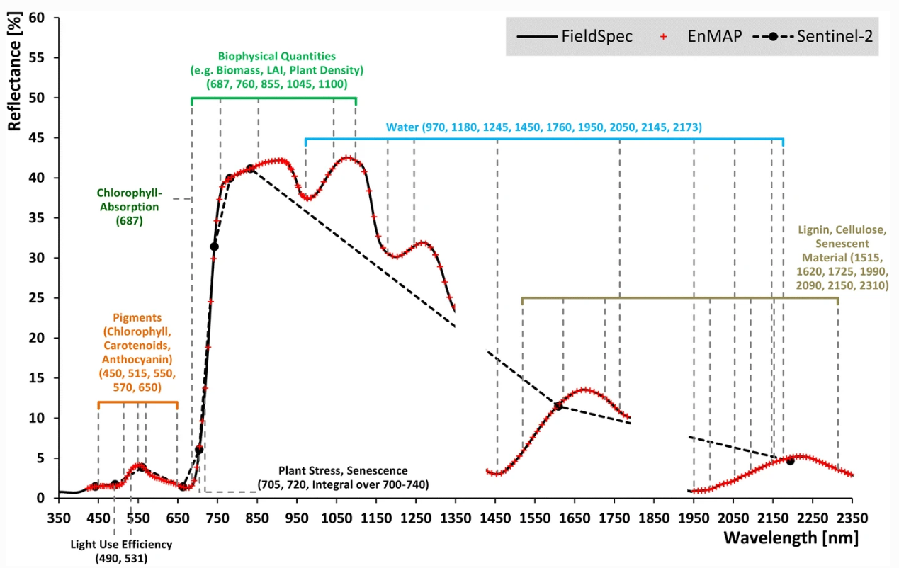
Optical remote sensing enables the deduction of various vegetation-related characteristics, including biochemical properties (e.g., pigments, water content), structural properties (e.g., leaf area index (LAI), biomass) or process properties (e.g., light use efficiency (LUE)). The ability to deduce these characteristics depends on the ability of a sensor to resolve vegetation spectra. Hyperspectral sensors capture spectral information in hundreds of narrow and contiguous bands in the VIS, NIR and SWIR, and, thus, resolve subtle absorption features caused by specific vegetation constituents (e.g. anthocyanins, carotenoids, lignin, cellulose, proteins). In contrast, multispectral sensors capture spectral information in a few broad spectral bands and, thus, only resolve broader spectral features. Still, multispectral systems like Sentinel-2 have been demonstrated to be useful to derive valuable vegetation properties (e.g., LAI, chlorophyll).

Vegetation spectrum in hyperespctral (ASD FieldSpec4, EnMAP) and multispectral (Sentinel-2) resolution as well as characterictic spectral features caused by various constituents and processes (absorption lines shown as grey dashed lines) (Source: Hank et al. 2018).

Vegetation Indices

A vegetation index (VI) represents a spectral transformation of two or more bands of spectral imagery into a singleband image. A VI is designed to enhance the vegetation signal with regard to different vegetation properties, while minimizing confounding factors such as soil background reflectance, directional, or atmospheric effects. There are many different VIs, including multispectral broadband indices as well as hyperspectral narrowband indices.

Spectral transformations

Spectral indices have the advantage of being simple, but the disadvantage of disregarding information of the spectral feature space. Linear transformations, such as the Tasseled Cap Transformation, Principle Component Analysis (PCA) on the other hand make use of all information, but can be substantially more difficult to interpret thematically.

Data transformations apply some function \(f\) to transform an input \(x\) to an output \(f(x)\), motivated by emphasizing certain information in the data (vegetation, water, soil, etc.) and simultaneously reducing the dimensionality (e.g. 6-band to single-band image). In the remote sensing context, one such common linear transformation is called the Tasseled Cap Transformation (TC) which already comes with a prespecified focus on certain information regarding spectral brightness, greenness and wetness.

In case you are interested in exploring more spectral indices please see this exhaustive list of indices.

NDVI

Most of the multispectral broadband indices make use of the inverse relationship between the lower reflectance in the red (through chlorophyll absorption) and higher reflectance in the near-infrared (through leaf structure) to provide a measure of greenness that can be indirectly related to biochemical or structural vegetation properties (e.g., chlorophyll content, LAI). The Normalized Difference Vegetation Index (NDVI) is one of the most commonly used broadband VIs:

\[NDVI = \frac{NIR - RED}{NIR + RED}\]

The NDVI calculation results in an singleband grayscale image, with a potential range of NDVI values between -1 and 1. For all possible input combinations of \(RED\) and \(NIR\) we observe the following NDVI values:

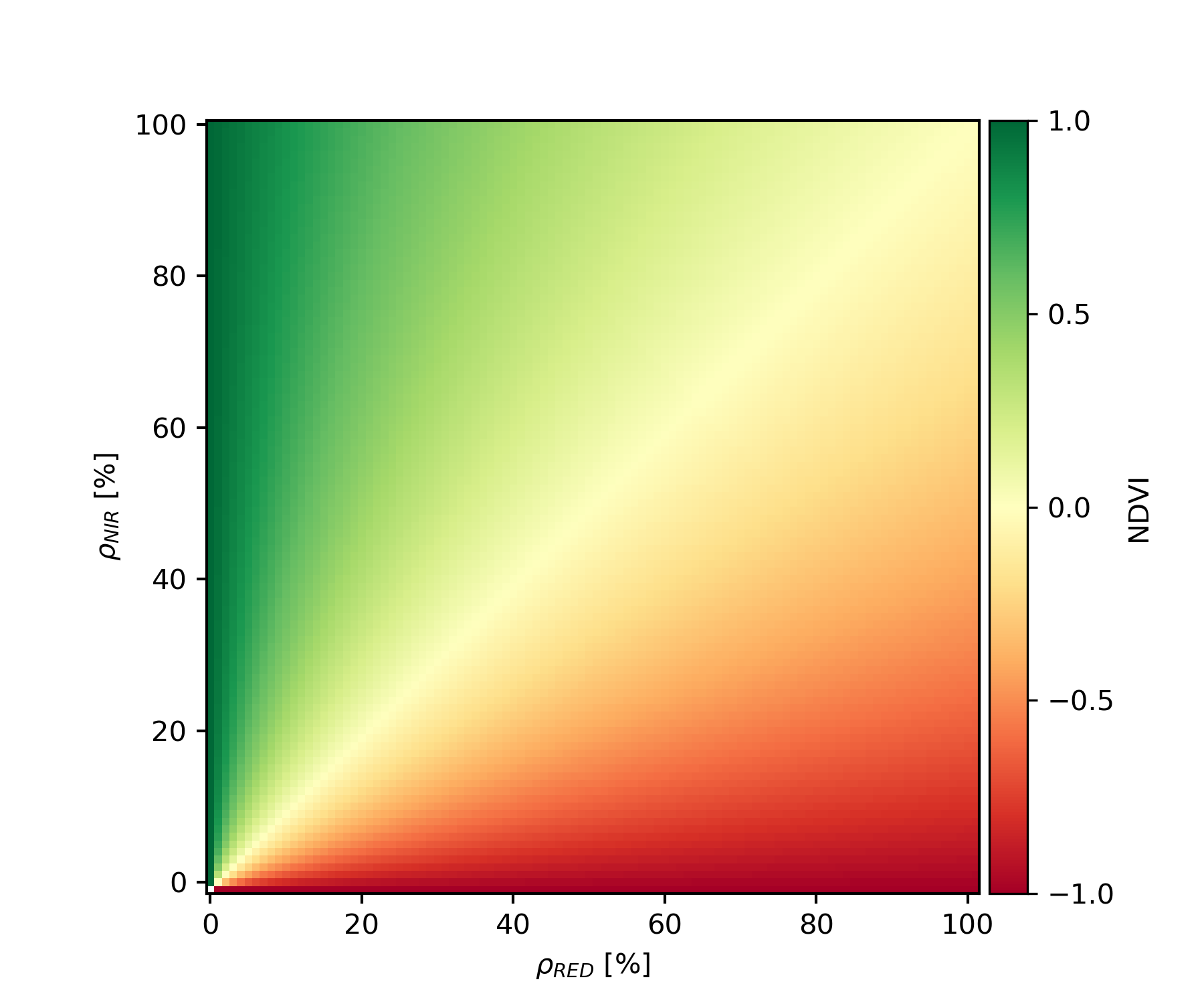
NDVI response curve for NIR and RED reflectance

The NDVI is a great proxy for photosynthetic activity, leaf vitality, vegetation density and canopy structure. It is, however, not a biophysical variable. Nevertheless, because of its relation to vegetation density and structure, the NDVI may be used to estimate biophysical parameters such as the Leaf Area Index (LAI).

Exercise 1
Take a look at the NDVI formula above. Think about the (general) spectral behaviour of 1) water, 2) soil, and 3) vegetation (take a look at last week’s plots if needed). Roughly which NDVI values would you expect to observe for these surface types?

Water: If it does not contain photosynthetic organisms like plankton, the light is stronger absorbed in the NIR than in the RED, thus values < 0 are to be expected. Soil: Usually characterised by increasing reflectance with increasing wavelength, yet jumps between RED and NIR are rather subtle, thus values around 0.1-0.4 are to be expected. Vegetation: If strongly photosynthetically active, the red-edge characteriseses are marked jumpt from RED to NIR, thus values >0.5 are to be expected.

Sentinel-2 subset of Berlin-Koepenick represented as false-color RGB composite (left) and as NDVI grayscale image (right).

Next, we will take a look at how to calculate the NDVI in R. We will see there are many options, but first we consider the simplest when dealing with only one image:

Exercise 2
Start by reading in your Sentinel-2 image from the last sessions (the one that is scaled and reprojected) into R. In Session 3 you applied simple arithemtic to scale your data. Along these lines, we can now also calculate the NDVI by simply treating the correct bands of the SpatRaster as inputs to our formula. An example:

# two hypothetical measurements in the red and nir
red <- 0.045  # 4.5%
nir <- 0.382  # 38.2%

ndvi <- (nir-red)/(nir+red)
print(paste0("NDVI: ", round(ndvi, 3)))

## [1] "NDVI: 0.789"

In the above example we simulate the calculation on a single pixel. Now calculate the NDVI for the entire image:

# ...

# print and plot resulting single-band NDVI
print(ndvi)
plot(ndvi)

img_s2  # our 6-band Sentinel-2 image
# option 1
red <- img_s2$RED  # or index: img_s2[[3]]
nir <- img_s2$NIR  # or index: img_s2[[4]]
ndvi <- (nir-red)/(nir+red)
# option 2
ndvi <- (img_s2$NIR-img_s2$RED)/(img_s2$NIR+img_s2$RED)
# print and plot resulting single-band NDVI
print(ndvi)
plot(ndvi)

Remember functions? Of course! - You work with them all the time, like rast(), plot(), … But we can also create our own functions in R: User-defined functions.

Calculations such as the NDVI are a good example for tasks we do repeatedly for different images. So let’s see how we can create a function which allows us to calculate the NDVI given an input image.

User-defined functions in R

User-specified functions come in handy whenever a certain chain of instructions need to be repeated or generalized. A function is a set of statements organized together to perform a specific task. Using functions greatly enhances code structure as it improves the clarity and readability of your script.

Function arguments are provided in round () brackets following the function class. Between {} stands the function body which contains the collection of statements which should be executed when calling the function. At the end there is usually an output, specified within return().

Let’s create a simple “coin-flip” function:

# coin-flip function - 
coin_flip <- function(n_flips=1) {
  flip_result <- sample(c("Heads", "Tails"), size=n_flips, replace=TRUE)
  return(print(flip_result))
}

# single coin flip
coin_flip()

## [1] "Heads"

# 5 coin_flips
coin_flip(5)

## [1] "Tails" "Tails" "Tails" "Tails" "Tails"

Let’s implement our own NDVI function we can use in the future.

Exercise 3
Create a function called calc_ndvi which expects two arguments as inputs: the red and nir single-band images, and returns a single-band NDVI image. After checking the result for correctedness, export it to disc or take a look at the optional exercise below.

calc_ndvi <- function(red, nir) {

}

Advanced (optional): Expand the functionality of calc_ndvi to provide a filename as function argument which - if provided - saves the resulting NDVI to disc. Ideally scaled and in 16bit signed (+ and -) integer (INT2S)

calc_ndvi <- function(red, nir, filename=NULL) {
  # your ndvi calculation from above
  # ...

  # check if filename is not equal (!) to NULL; i.e.
  # a filename was provided to the function
  if (!is.null(filename)) {
    # scale

    # export image to disc

  }
  
  # your "return" from above
  # ...
}

calc_ndvi <- function(red, nir) {
  # your ndvi calculation from above
  ndvi <- (nir-red)/(nir+red)
  names(ndvi) <- "NDVI"
  return(ndvi)
}

calc_ndvi <- function(red, nir, filename=NULL) {
  # your ndvi calculation from above
  ndvi <- (nir-red)/(nir+red)
  names(ndvi) <- "NDVI"
  # check if filename is not equal (!) to NULL; i.e.
  # a filename was provided to the function
  if (!is.null(filename)) {
    # scale
    ndvi <- ndvi * 10000 # prepare for integer export
    # export image to disc
    writeRaster(ndvi, filename=filename, datatype="INT2S")
  }
  # return ndvi as SpatRast object
  return(ndvi)
}

Assignment

The senate of Berlin would like to have a first short assessment of the amount and condition of the urban vegetation within city borders. Specifically, the senate would like to get a first idea how much of the area is covered by vegetation. Based on the NDVI, they want you to assign to each pixel if it represents vegetation cover, or not. For instance, you could say that everything above a NDVI of 0.85 represents full vegetation cover, while everything below 0.85 does not.

Greenness of Berlin: Conceptual implications

Before you get started, you explain to the senate that finding a NDVI threshold which separates vegetation from non-vegetation is not a straightforward task. Think about the data you are using, and recap the theory on the NDVI from the lecture to list at least 3 points that complicate finding a universal, exact threshold.

Greenness of Berlin: Land cover - NDVI relationship

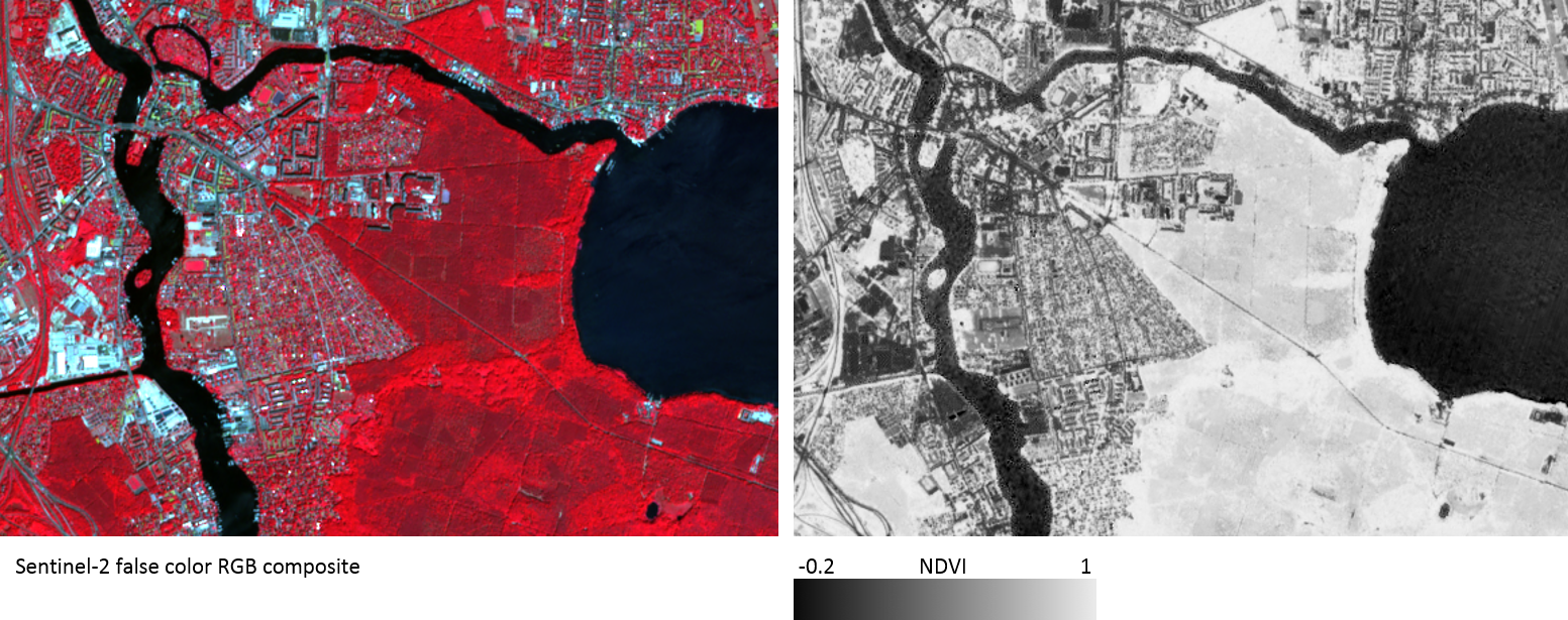
Display the NDVI as grayscale image and the Sentinel-2 image as true-colour composite in QGIS. Simultaneously, have the NDVI image ready-for-analyses in R.

First, use the Identify cursor location values functionality and the histogramm in QGIS to answer the following questions:

What is the range of NDVI values for the entire image (min, max), and which land cover types are likely located at these extrema?
What are typical NDVI values for 1) built-up, 2) vegetation (grassland, broadleafed, coniferous, cropland), and 3) water? (Tipp: Visit some of the land cover points you sampled in Session 5 and visually intepret your NDVI image in QGIS to get a rough estimate how these 3 surfaces behave)

Greenness of Berlin: A first map

The senate would like you to create a vegetation map based the area covered by leafes (the Leaf-Area-Index, LAI) approximated via its relationship to the NDVI (Lecture slide 14). The map should label every pixel as vegetation where at least 3 square meters are covered by leafes (LAI = 3). This map hence focuses on rather densely covered pixels. To identify the NDVI threshold for creating this map, take a look at the graph on lecture slide 14, showing the general LAI-NDVI relationship.

Why is finding such a threshold based on this graph difficult and not ideal?
Can you explain if we could attempt to separate even denser canopies (LAI > 3) from each other? Why is this difficult?

Use a best estimate of the NDVI threshold (e.g. mean in plot) to approximately separate pixels with LAI > 3 and LAI <= 3. Once you have your threshold, you can use the following code to create a simple binary map containing 1 for vegetation and 0 for non-vegetation:

# 'ndvi' is your NDVI image
# 'ndvi_threshold' is your chosen value to separate the cover
ndvi_threshold <- 

# Use "greater than" > to check for every pixel if the value is greater than 
# the ndvi threshold; If true, "vegetation" will contain 1, if false, "vegetation"
# will contain 0
vegetation <- ndvi > ndvi_threshold
plot(vegetation)

# write your map to disc
writeRaster(vegetation, filename = )

Take a quick look at your result in QGIS. Compare the result to Google VHR imagery and your Sentinel-2 image. Are you satisfied with the product? Does the map allow you to get a good apprximation of vegetation presence within Berlin?

6. Vegetation properties and indices