7. Image classification - Decision Trees

Learning goals

Understand the principle idea of decision trees
Develop a set of rules for classifying Berlin land cover categories
Implement a decision tree in R

Image classification: Decision trees

Image classification is a key component of many remote sensing applications when deriving thematic information from measured reflectance. The choice which classification algorithm to use relates - amongst other points - to the 1) type of the classification problem (i.e. number and type of classes), 2) the (statistical) assumptions, 3) the number of input features (e.g. number of spectral bands), 4) or the computational performance needed. In simple words: A one fits all solution does not exist (if you are interested to find out more by yourself, google “No Free Lunch Theorem”).

Decision trees (DT) are arguably one of the most intuitive classifiers and provide a good entry point into the realm of (image) classification.

Decision Trees
Decision Trees (DTs) are constructed from a sequential set of decision-rules branching out into a tree-like structure. DTs convert inputs (such as measured spectral reflectance) into thematic (classification) or continuous (regression) outputs (e.g. land cover classes). This works by sequentially splitting each input according to the binary (true/false) decisions-rules.

Take a look at the above DT as an example, starting at the top. The boxes are referred to as ‘nodes’. Each node contains a binary decision which evaluates an input to be either TRUE (1) or FALSE (0) based on logical operators (>, <, =, …) (see yellow box down below for details on logical operators). The path downward the tree continues to the next node based on the decision for a given data point (e.g. a pixel). In the above example, a final decision is reached after at most three nodes. Depending on the classes of interest and the spectral information available, DTs can become very complex and “deep”, i.e. use many different features (e.g. bands) and contain many nodes.

According to this DT, every pixel having an NDVI of < 0.6 and a SW1 reflectance of < 5% belongs to the class ‘water’. Applying this very simple DT to the Sentinel-2 image of Berlin already produces meaningful classification results for the water class.

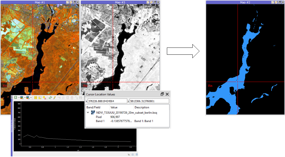
The resulting map shows us ‘water’ pixels against all other ‘unclassified’ pixels. As indicated by the DT above, more decision rules are needed to discriminate the other unclassified pixels and thereby produce a complete land cover map from the image.

Logical/Boolean Operators

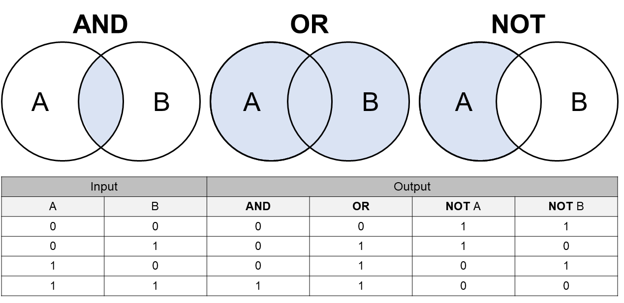
Boolean Logic is a form of algebra that forms the basis for mathematical set and database logic. It is binary as it only involves two states, 0 or FALSE and 1 or TRUE. Boolean or also called Logical Operators are the fundamental building blocks of Boolean Logic and consist of the words And, Or and Not. Using this logic, we can evaluate the output for a given set of inputs, e.g. two inputs A and B:

Logical Operators AND, OR, and NOT.

Implementing a Decision Tree in R

In the following exercise, we first want to implement the above displayed DT in R using logical operators.

Exercise 1

# INPUT
img_s2  # your sentinel-2 SpatRast
ndvi  # your NDVI raster

# DECISION TREE
# set rules at each node; each results in two outputs, one TRUE, one FALSE
# root node "N1"
N1_T <- ndvi < 0.6 # TRUE (value = 1) for every pixel meeting the condition and FALSE (0) otherwise
N1_F <- !N1_T # the "!" operator inverts the above statement: 1s in N1_T become 0s, 0s become 1s

Take a look at the outputs N1_T and N1_F. Make sure you comprehend the output. Which classes are now ideally stored as 1s in N1_T and N1_F, respectively?

Next we want to finalise the left branch of the above decision tree. As you can see node “N2A” splits into the classes or leaf nodes “water” and “built-up”. Take a look at your plots from Session 5 which show the various reflectance spectra of the different thematic land cover classes. Based on these identify one suitable threshold in a specific band that could help separate water from built-up. (Please remember that reflectance is usually expressed as a fraction between 0.0 and 1.0. The values of the image are scaled by 10000.)

# nodes tree layer 2 left branch "N2A"
N2A_T <- 
N2A_F <- !N2A_T

Once the left branch is split into the leaf nodes “water” and “built-up” you can start filling your final land cover map which is supposed to contain the classID integers for each pixel in the end. We can create an empty raster based on the Sentinel-2 image and then based on the decision rules, index pixels and fill them with the correct classID values:

# OUTPUT
# create empty raster in which to fill land cover ID's
LC <- rast(img_s2[[1]], vals=0)
LC
print(LC)  # only 0s, but same extent, resolution, CRS

# we use '*' as the logical operator "AND", i.e. only pixels in the classification layer where 
# condition 1 AND condition 2 are TRUE will be set to a user defined value (here = 6, "class-id" of water)
LC[N1_T*N2A_T] <- 6  # classID = 6; water;

LC[] <- 1  # classID = 1; built-up;

Write the intermediate LC map to disc. Open the map and the Sentinel-2 image in QGIS.

Discuss the classification result:

Are the decision rules and values for the water/built-up separation well selected?
Would you recommend an alternative rule set for classifying water?

Assignment

Expand the DT

Expand the existing DT to classify the remaining classes according to the following structure.

Use the code snippet below to develop new decision rules for the empty nodes (‘…’). Please get familiar with the code and underlying commands by carefully reading through the #explanations.
Update the code sections “set rules for nodes” and “Create the decision tree for classification” with your modifications.

# INPUT
img_s2  # your sentinel-2 SpatRast
ndvi  # your NDVI raster

# DECISION TREE
# set rules at each node; each results in two outputs, one TRUE, one FALSE
# root node "N1"
N1_T <- ndvi < 0.6 # TRUE (value = 1) for every pixel meeting the condition and FALSE (0) otherwise
N1_F <- !N1_T # the "!" operator inverts the above statement: 1s in N1_T become 0s, 0s become 1s

# nodes tree layer 2 "N2"
N2A_T <- 
N2A_F <- !N2A_T
N2B_T <- 
N2B_F <- !N2B_T

# nodes tree layer 3 "N3"
N3_T <- 
N3_F <- !N3_T

# OUTPUT
# create empty raster in which to fill land cover ID's
LC <- rast(img_s2[[1]], vals=0)
LC
print(LC)  # only 0s, but same extent, resolution, CRS

# we use '*' as the logical operator "AND", i.e. only pixels in the classification layer where 
# condition 1 AND condition 2 are TRUE will be set to a user defined value (here = 6, "class-id" of water)
LC[N1_T*N2A_T] <- 6  # water
LC[] <- 1  # built-up/soil
LC[] <- 2  # grassland/cropland
LC[] <- 3  # broadleafed
LC[] <- 4  # coniferous

Discuss the resulting classification critically, i.e. mention well-delineated classes as well as prominent errors
What could be key weaknesses/strength of such a user-defined decision tree method?

Submission

Please upload your the classification as .tif file and a separate .pdf file containing your knitted .Rmd-script, the classification as visualized image (map + legend) and the discussion in bullets to moodle.