8. Image classification - Random Forests

Learning goals

Get introduced to a supervised classification workflow
Perform a Random Forest classification

Image classification: Random Forests

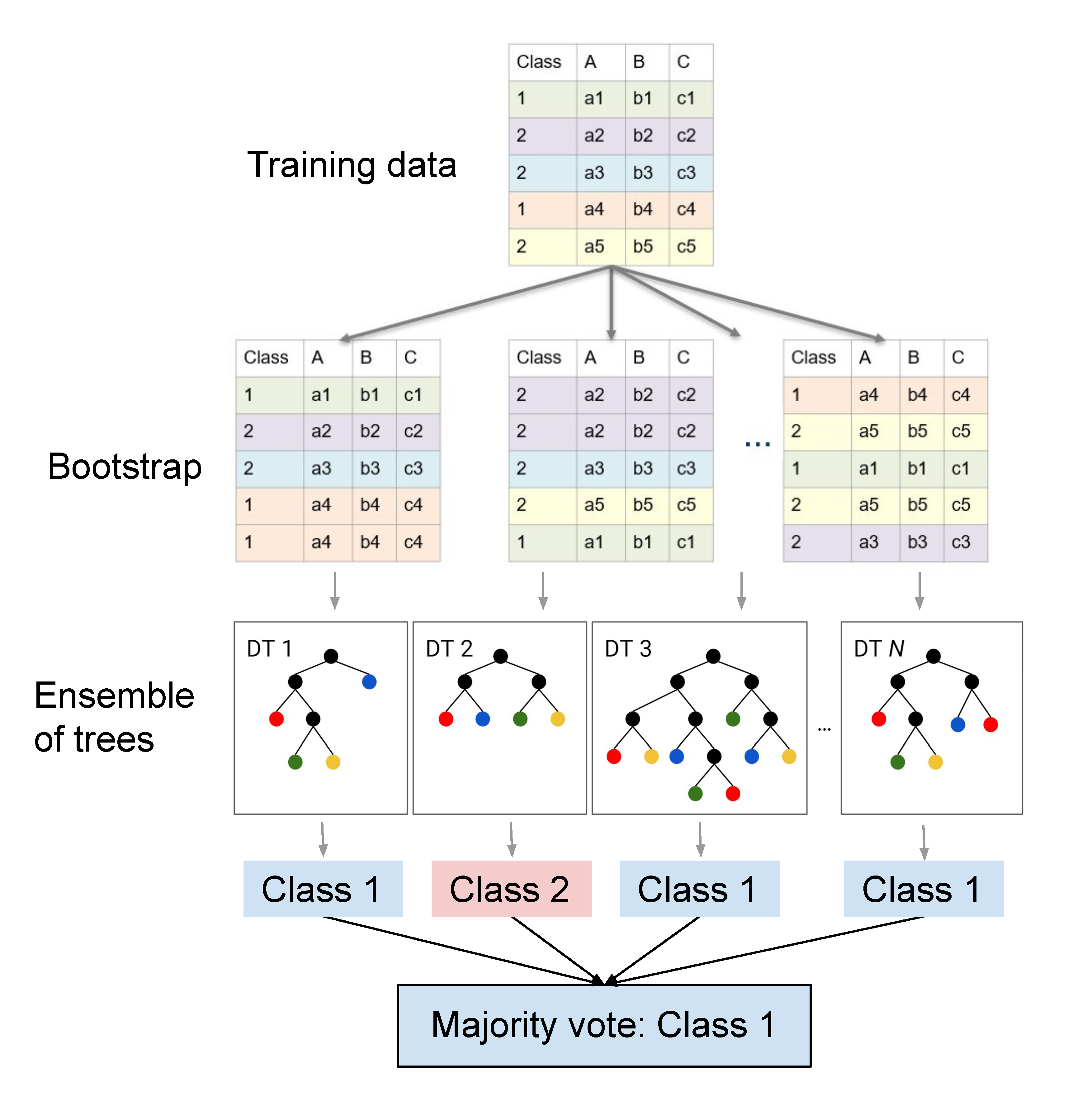
The Random Forest (RF) algorithm (Breimann 2001) belongs to the realm of supervised classification algorithms. RFs builds upon the concept of decision tree learning presented in the last session. The RF relies on many self-learning decision trees which in their sum make up a “forest”. The idea behind using not one, but many decision trees (i.e. an ensemble) is that many base learners can come to a more accurate and robust decision compared to a single DT. Different from the manual (expert-based) definition of decision rules we defined last week, the RF uses self-learning decision trees. This “self-learning” involves automatically defining rules at each node based on a training dataset for which feature inputs and labels are known.

These “optimal” decision rules are calculated statistically. One way to define the optimal split given a set of input features and training points, would be trying to minimize the heterogeneity (i.e. class-mixtures) of the two resulting subsets of data after splitting. A frequently used measure of heterogeneity in decision tree learning is the Gini impurity, stemming from the concept of entropy in information theory. To identify the best split at each node, the subsequent Gini impurity index is calculated for each potential split of the data and the one split with the least heterogeneity is chosen.

The term “Random” in RFs relates to two major layers of randomness in the learning process: First, RFs use a bootstrapped sample (i.e., random sample with replacement) of the original training dataset for growing each individual decision tree. Accordingly, the training set for the trees (in the vast majority of cases) are different from one another. This may appear odd at first, but this greatly reduces the correlation between trees and improves the generalisation of the predictions. The second random component is a random selection of the features (e.g. spectral bands) considered at each node. Accordingly, the splits are determined for varyinig features, also heping with decorrelating the trees.

Many trees may produce different class labels for the same data point. The final class assignment of each image pixel is ultimately chosen based on the majority vote among all trees in the RF.

Schematic structure of the RF algorithm

Random Forest
If you want to know more details on how decision tree learning and the Random Forest algorithm work, you may take a look at the materials of our Master’s course.

Random Forest classifier in practise

We have identified the following six classes:

`classID`	Land Cover Class
1	Built-up (urban, sealed, soil, …)
2	Grassland/Herbaceous
3	Broadleafed woody vegetation
4	Coniferous woody vegetation
5	Cropland
6	Water

Our goal today is to predict the 2019 land cover for the greater area of Berlin using the Random Forest classifier. For this we will need:

Training data: The point vector file (.gpkg) for which you have identified the land cover at selected pixel locations
Image features: The image data we want to use to train the classifier and finally predict the land cover (Sentinel-2 scene)

With the data prepared, we need to do the following to create a supervised classification map:

Data preparation: Extract the feature values of the Sentinel-2 image at the training point locations into a data.frame
Model building: Supply the feature-label data.frame to the randomForest-function
Prediction: Classify the entire Sentinel-2 image using the image data, model, and the terra::predict function

Exercise 1
First we need to make sure the randomForest package is installed:

# install the randomForest package
install.packages('randomForest')
# load the package to get access to the package's routines/functions in your environment
library(randomForest)

Data preparation
Load the vector file containing your training data points using terra::vect(). Create a rast()-stack containing your 6 Sentinel-2 bands and the NDVI. Next, use extract() to create a data.frame containing the classID from the vector and the band names from the Sentinel-2 image as columns. Make sure that that you remove any other columns which are not meaningful predictors.

df <- data.frame(
  terra::extract(x=, y=, bind=TRUE)
)
df

Model building
As we want to train a classifier (and not a regressor), the randomForest() function expects the dependent variable (here: classID) to be of type factor. Use as.factor() to convert the classID column to factor.

df$classID <- as.factor(df$classID)

Like most models, the RF algorithm cannot deal with missing data (NA). Remove potential NAs from the data.frame (if there are any at all in the image) using na.omit() on the data.frame:

df <- na.omit(df)

Now we can train the model by supplying the data.frame to the randomForest-function:

rf_model <- randomForest(classID~., df, ntree=500)
rf_model

That’s it. Model trained and ready for prediction. Ignoring the very important step of evaluating the model for the moment. What just happened is what was described above. The classifier used self-learning decision trees to build a forest of 500 trees. Take a look at the output by printing rf_model to your R console.

What is the expected out-of-sample overall accuracy (OOB estimate of error rate)? How low/highare the error rates per class? Are there differences between classes?

Prediction
To create a classification map we simply predict the label for each pixel using the trained model and the image data:

rf_prediction <- terra::predict(img_s2, rf_model, na.rm=TRUE)
rf_prediction
plot(rf_prediction)

Last, write the prediction result to disc and evaluate the map in QGIS.

Assignment

In the assignment you will revise the above Random Forest model by 1) gathering additional data if needed and 2) use multitemporal imagery to allow for better separability of classes.

Additional NDVI features at different seasons

Some classes like cropland and different forest types are better separable when capturing their distinct land surface phenology by using images from more than one point in time. Therefore, we provide you three more Sentinel-2 scenes (download here):

20190216_LEVEL2_SEN2A_BOA_berlin.tif: Sentinel-2 scene from the 16th February 2019
20190422_LEVEL2_SEN2A_BOA_berlin.tif: Sentinel-2 scene from the 22nd April 2019
20190921_LEVEL2_SEN2A_BOA_berlin.tif: Sentinel-2 scene from the 21st September 2019

Open the scenes in QGIS and make yourself familiar with the data. The band arrangement is identical to the July scene you hve been working with the last weeks.

Next, the goal is to build a new Random Forest model which now also contains the additional information from different points in time. However, scince using all bands from all four images is not necessary and rather contains a lot of redundant information, the idea is to calculate the NDVI for the three new scenes, and only add the three NDVI images to your exisiting raster stack you used above.

Once you have your raster stack containing the 6 bands + NDVI from July, as well as the NVI from the three other dates (= 10 band stack), repeat the classification workflow from above: Data preparation, model building, and prediction.

The bandnames of all images are identical (BLU, GRN, RED, …). However, in the data.frame and model, they have been renamed because there cannot be duplicate column names in data.frames. Your raster stack will, however, have duplicate names (check names() on your stack). Accordingly, rename your image band names to the same names as the columns of your data.frame before you can predict your model. For instance:

# get column names from data.frame (after extracting training data o new stack)
new_bandnames <- names(df)[2:length(names(df))]
names(stack) <- new_bandnames  # stack is your new 10 band raster

Evaluate the output of your new model: What is the expected out-of-sample overall accuracy (OOB estimate of error rate)? How low/highare the error rates per class? Are there differences between classes? How does it compare to your first model from Exercise 1? lso visually assess the qualitative appearance of the final product in QGIS? Identify three regions/pixels which represent mixed land cover. How does the classify behave for these regions?

If you think you can increase model performance, expand your training dataset by collecting further training points for the “problematic classes”. For instance, consider including mixed pixels that are dominated by impervious surfaces (> 50%) into the “built-up” class. Repeat the RF classification with the expanded training points and critically evaluate the revised classification result. Repeat the revision procedure until you reach a satisfying final classification result. Note that a certain degree of confusion between thematic classes most likely remains due to the overlap of spectral classes of different thematic classes.

Submission

Please upload the final classification result (map incl. legend) in R and the discussion points as knitted html/pdf onto moodle.