5. Spectral properties II - Imagery

Learning goals

• Explore the spectral appearance of different surface types in multispectral imagery
• Learn the difference between spectral and thematic classes
• Sample spectral reference data for different land cover classes

It is time to recall our first major goal: Creating a land cover map of Berlin. Now that we have a basic toolset to handle satellite data in R and QGIS, and experienced in the laboratory how different surface types behave spectrally, we will now translate what we learned in the laboratory to satellite images and see how different land cover types behave when measured from space. From this we will gain insights into the basic principle that underlies land cover mapping using optical remote sensing, moving us one step closer to creating our own land cover map.

Spectral Signatures

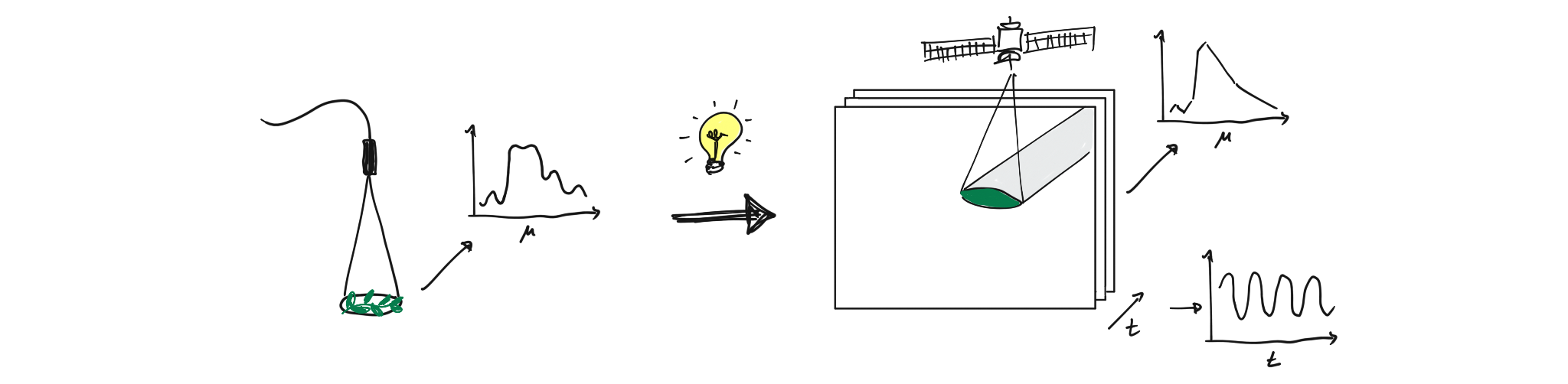
Last week you took a closer look at the spectral dimension of remote sensing data. When the sunlight travels through the atmosphere and strikes surface materials on the ground, certain wavelengths are absorbed while others are reflected, transmitted or emitted. Depending on the surface material the energy interacts in a unique way. This material-specific reflectance-absorbance behaviour is known as its spectral signature.

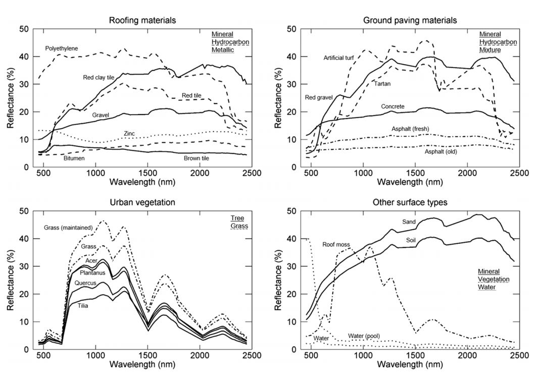
The unique spectral behaviour of materials is controlled by their structural properties (e.g. roughness), the chemical composition (e.g. water content), as well as the illumination- and recording-geometry between sensor and target object. When focusing on vegetation, for instance, optical remote sensing enables the deduction of various vegetation-related characteristics, including biochemical properties (e.g., pigments, water content), structural properties (e.g., leaf area index (LAI), biomass) or ecological processes (e.g., light use efficiency (LUE)). When our goal is to differentiate among different surface types or land cover, we can also make use of these unique spectral fingerprints. In an urban environment such as Berlin we find a multitude of surface types:

Spectral library of urban surface spectra ordered by land cover type as extracted from an HyMap image at 3.6 m resolution from Berlin, Germany (Source: van der Linden et al. 2018)

As you already know, the ability of a sensor to deduce these spectral characteristics depends on the spectral and radiometric resolution. In the example above, the hyperspectral sensor enables the differentiation of surface types which in multispectral data might be difficult to separate. When we compare the the spectral detail which can be resolved between hyperspectral sensors in the lab (ASD FieldSpec4) and from space (EnMAP) to multispectral measurements (Sentinel-2):

Vegetation spectrum in hyperespctral (ASD FieldSpec4, EnMAP) and multispectral (Sentinel-2) resolution as well as characterictic spectral features caused by various constituents and processes (absorption lines shown as grey dashed lines) (Source: Hank et al. 2018).

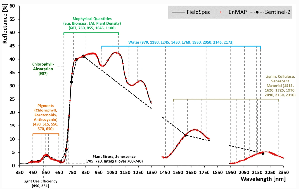
We can see that (1) Hyperspectral sensors capture spectral information in hundreds of narrow and contiguous bands in the VIS, NIR and SWIR, and, thus resolve subtle absorption features caused by specific vegetation constituents (e.g. anthocyanins, carotenoids, lignin, cellulose, proteins). (2) Multispectral sensors capture spectral information in a few broad spectral bands and, thus, only resolve broader spectral features.

Despite this, multispectral systems such as Sentinel-2 are very much capable of deriving valuable information on surface composition and state, since key absorption and reflectance patterns are also captured in the fewer bands of Sentinel-2. A key reason we work with multispectral medium resolution (spatial) sensors like Sentinel-2 or the Landsat family, is their superior temporal resolution and global coverage, providing dense image time series allowing, for instance, capturing the phenology of vegetation at a high level of detail.

From Reflectance to Land Cover

The unique spectral behaviour of different surface types builds the foundation for mapping land cover, i.e. assigning pixels a categorical label (thematic class / land cover) based on the spectral measurement of a given pixel. Thus our overarching goal of mapping land cover in Berlin and assessing urban greenness draws exactly on this principle.

With the target goal in mind, we commonly create a class catalogue in which we identify the land cover classes we would like to map. For instance, such a land cover class could be labeled built-up, covering artificial, human constructed and sealed surfaces such as asphalt, roofs, concrete, etc. Although thematic land cover classes share similar spectral signatures due to compositional similarity, they can nevertheless exhibit substantial variance in their spectral behaviour. First, because of the above mentioned influences on the spectral behaviour (i.e. structure, composition, geometry), and second, because the within-class spectral variance can be arbitrarily high depending on the class definition.

The theoretical feasibility of separating land cover classes is governed by …

… the spectral and radiometric detail provided by the sensor define the data baseline. The higher the spectral resolution (incl. the number of bands) the more potentially useful information is available to seperate the classes. Take a look at the urban vegetation spectral signatures in the plot above. Imagine we only had data from the visible domain of the electromagnetic spectrum. We can see that information in the infrared regions is highly valuable and better separates the different species compared to the visible reflectance.

… the spectral (dis)similarity between classes. If objects have a similar to very identical behaviour towards light, then even capturing the best spectral and radiometric detail will not be of great help.

Develping a class catalogue

You have learned that different surfaces have unique spectral signatures which potentially allows us to differentiate them in our remotely sensed imagery. For our goal of mapping land cover of Berlin, we have identified the following six thematic classes:

classID	Land Cover Class	Sub-classes
1	Built-up (urban, sealed, soil, …)	…
2	Grassland/Herbaceous	…
3	Broadleafed woody vegetation	…
4	Coniferous woody vegetation	…
5	Cropland	…
6	Water	dark deep water, shallow sediment loaded water, …

This definition will allow us to 1) separate the different target vegetation types (grass, broadleafed, and coniferous trees) from background classes (built-up, cropland and water). Simultaneously, this land cover definition can be considered complete, i.e. we do not omit major surface types which could not be assigned to any of the categories.

Exercise 1
A colleague of yours has started collecting point locations of Sentinel-2 pixels covering the above land cover types. They are stored in this .gpkg-file. Open the file in QGIS and inspect its attribute table (Right click > Open Attribute Table). Unfortunately, the row-entries of the classID-column are empty and the description shows six different letters but we do not know to which land cover they belong to.

In order to get familiar with the spectral behaviour of the surface types and allocate the sampled points to the correct land cover (classID), you will now create spectral signature plots similar to last week’s laboratory session. This time these plots will show the spectral values obtained from the Sentinel-2 image. To do this, we will have to:

1. Read the scaled and reprojected Sentinel-2 image from last week’s assignment into R (download)
2. Read in the .gpkg vector file into R which contains the initial point locations of the land cover types
3. Extract the spectral reflectance values of the Sentinel-2 data at the point locations into a table/dataframe
4. Plot the spectral signatures according to their unique description value
5. Interpret the spectral plots to assign them to the correct classes
6. Write the manipulated SpatVector to disc

The following code lists the necessary steps and outlines some of the code needed to accomplish this.

1) Read the Sentinel-2 image from last week’s assignment into a SpatRaster object.

# load required library
library()
# create a string/character variable containing the path to the file
path_s2 <- 
# create a SpatRast variable using the path variable
img_s2 <- 
names(img_s2) <- c("BLU", "GRN", "RED", "NIR", "SW1", "SW2")
# verify it worked
print(img_s2)

2) Read in the .gpkg vector file into R which contains the initial point locations of the land cover types

Visit the terra-package website to learn how to read-in the .gpkg as a SpatVector into R.

# create a string/character variable containing the path to the file
path_landcover <- 
# create a SpatVector variable using the path variable
landcover <- 
# verify it worked
print(landcover)

# plot Sentinel-2 image and vector points
plotRGB(img_s2, r=6, g=4, b=3, stretch="lin")
points(landcover)

3) Extract the spectral reflectance values of the Sentinel-2 data at the point locations into a table/dataframe

Extract values from a SpatRaster for a set of locations can be achieved using the extract() function of the terra package.

# extract the raster values at each point and append as attribute to SpatVector
spectral_signatures <- terra::extract(
  x=,
  y=,
  bind=TRUE
)
# convert to data.frame
df <- data.frame(spectral_signatures)
df

4) Plot the spectral signatures according to their unique description value

Now that we have extracted the image-based spectral signatures at each point location, we can plot them coloured by description.

# create a vector of packages we need to load (and potentially install)
l_packages <- c("ggplot2", "tidyverse")

# loop over this vector and check if packages is already installed
# if not, then install / if yes, only load
for (p in l_packages){
  if(! p %in% installed.packages()){
    install.packages(p, dependencies = TRUE)
  }
  library(p, character.only = T)
}

# convert df to "long format" using "pivot_longer"
df$ID <- c(1:nrow(df))
df_long <- df %>%
  pivot_longer(cols = -c(classID, description, ID), names_to = "band", values_to = "value")
# check what the long format means
df_long

# currently, our band names are 'BLU', 'GRN', etc.
# let's save the actual wavelength in nanometers for better plotting
# we create a vector containing the integer central wavelength for each band
remap_dictionary <- c('BLU' = 490, 'GRN' = 560, 'RED' = 665, 'NIR' = 842, 'SW1' = 1610, 'SW2' = 2190)
# then we use match to create a new column 'wavelength' which gets filled with the correct 
# value based on the entry of 'band'
df_long$wavelength <- remap_dictionary[match(df_long$band, names(remap_dictionary))]

# plot each spectral signature; we create a plot window for each class ('description');
# we also colour according to 'description'; we group by 'ID' to get a single plot for each point
ggplot(df_long, aes(x = wavelength, y = value, group = ID, color = as.factor(description))) +
  geom_line() +
  scale_color_manual(values = c("red", "blue", "darkgreen", "purple", "green", "orange")) +
  facet_wrap("description") + 
  labs(title = "Spectral signatures",
       x = "Wavelength [nm]",
       y = "Reflectance [%]",
       color = "description") +
  guides(color = "none") + theme_bw()

5) Interpret the spectral plots to assign them to the correct classes

# dictionary-like mapping: 'description' letter to correct 'classID' integer
remap_dictionary <- c('e' = , 'f' = , 'j' = , 'o' = , 'p' = , 'z' = )

# use match to create a new column based on the dictionary
spectral_signatures$classID <- remap_dictionary[match(df$description, names(remap_dictionary))]
spectral_signatures

6) Write the manipulated SpatVector to disc

writeVector(spectral_signatures[,1:2], "data/landcover_berlin_2019_labeled.gpkg")

# load required library
library(terra)
# create a string/character variable containing the path to the file
path_s2 <- "data/Sentinel-2/SEN2A_BOA_20190726_stack_int16_repro.tif"
# create a SpatRast variable using the path variable
img_s2 <- rast(path_s2)
# verify it worked
print(img_s2)

# create a string/character variable containing the path to the file
path_landcover <- "data/landcover_berlin_2019.gpkg"
# create a SpatVect variable using the path variable
landcover <- vect(path_landcover)
# verify it worked
print(landcover)

# plot Sentinel-2 image and vector
plotRGB(img_s2, r=6, g=4, b=3, stretch="lin")
points(landcover, col="red", cex=1)

spectral_signatures <- terra::extract(
  x=img_s2,
  y=landcover,
  bind=TRUE
)

df <- data.frame(spectral_signatures)

l_packages <- c("ggplot2", "tidyverse")

for (p in l_packages){
  if(! p %in% installed.packages()){
    install.packages(p, dependencies = TRUE)
  }
  library(p, character.only = T)
}

# Convert to long format using gather (or pivot_longer in newer versions of tidyr)
df$ID <- c(1:nrow(df))
df_long <- df %>%
  pivot_longer(cols = -c(classID, description, ID), names_to = "band", values_to = "value")

# dictionary-like mapping: 'description' letter to correct 'classID' integer
remap_dictionary <- c('BLU' = 490, 'GRN' = 560, 'RED' = 665, 'NIR' = 842, 'SW1' = 1610, 'SW2' = 2190)

# use match to create a new column based on the dictionary
df_long$wavelength <- remap_dictionary[match(df_long$band, names(remap_dictionary))]

# plot each spectral signature; we create a plot window for each class ('description');
# we also colour according to 'description'; we group by 'ID' to get a single plot for each point
ggplot(df_long, aes(x = wavelength, y = value, group = ID, color = as.factor(description))) +
  geom_line() +
  scale_color_manual(values = c("deeppink3", "blue4", "darkgreen", "purple", "yellow4", "orange")) +
  facet_wrap("description") + 
  labs(title = "Spectral signatures",
       x = "Wavelength [nm]",
       y = "Reflectance [%]",
       color = "description") +
  guides(color = "none") + theme_bw()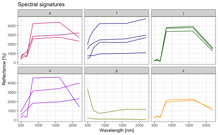

Interpretation in class.

# dictionary-like mapping: 'description' letter to correct 'classID' integer
# for correct classID, check land cover table above
remap_dictionary <- c('e' = 2, 'f' = 1, 'j' = 3, 'o' = 5, 'p' = 6, 'z' = 4)

# use match to create a new column based on the dictionary
spectral_signatures$classID <- remap_dictionary[match(df$description, names(remap_dictionary))]
spectral_signatures

writeVector(spectral_signatures[,1:2], "data/landcover_berlin_2019_labeled.gpkg")

By interpreting the above plots, we are faced with the difference between thematic and spectral classes:

Thematic vs Spectral Classes
In remote sensing, thematic land cover and land use classes consist of multiple spectral classes. Spectral classes are clusters of several surfaces which have similar spectral properties.

Imagine we would like to map a broad thematic land cover class labeled “vegetation”. The class “vegetation” should consider the spectral properties of various vegetation types, including trees, shrubs, grasses, etc. Similarly, a class labeled “forest” should consider the spectral properties of different forest types in the landscape, or an even more detailed class like “coniferous forest” should consider the spectral properties of potentially different species compositions and stand structures within this class. When defining a thematic class, it is therefore essential to consider the different spectral properties of the several surfaces, i.e. all spectral classes of a thematic class.

To illustrate what this means, consider we have measured the reflectance of several surfaces. For simplicity, we only plot the measured reflectance in the red and near-infrared region for our thematic classes:

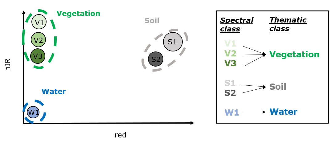
Our spectral measurements build spectral classes in this two dimensional feature space of red and near-infrared reflectance. Now, if all spectral classes of a thematic class are nicely separable from the spectral classes of the other thematic classes, the separability of the thematic classes is possible.

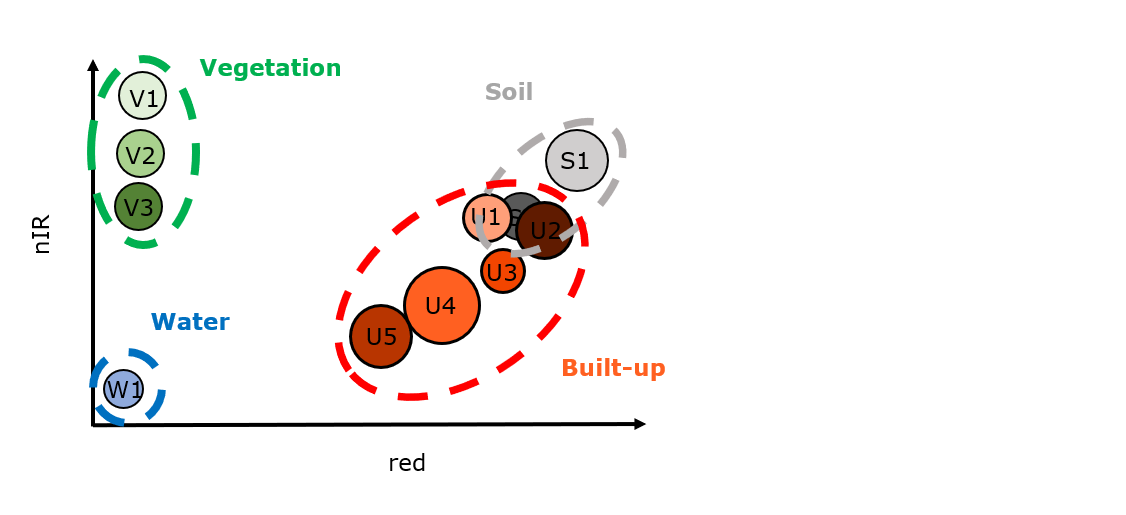
Sometimes, however, different thematic classes overlap spectrally. In this case, the separability of the thematic classes will decrease or they even may not be separable. In this case, the thematic classes share similar spectral classes. To illustrate this, we add a class “built-up” to the above class catalog:

As you can see, some of the measurements we grouped into the “built-up” class overlap with measurements from the “soil” class. Based on our measurements in the red and nIR, it will be difficult to impossible to separate between “soil” and “built-up” when we observe a pixel that falls in this overlap for which we do not know the land cover yet. Luckily, we have more bands and other tricks we will learn, but remember: Just a thematic differentiation of classes does not mean we can differentiate them spectrally.

Sampling reference data

Collecting spectral reference information is an essential step on your way to a classified map. We often call this type of reference data training data since it is used to train a model.

Training points for forest type classification and the resulting classification map output

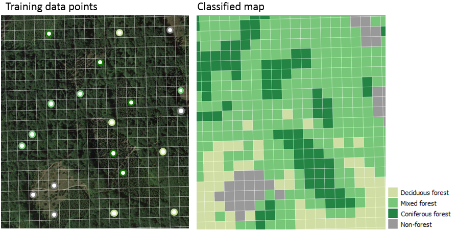
From the illustration above you can see that we select and label points (thus pixels) for which we can determine the land cover. Later we can use these reference samples to train a model which is capable of predicting land cover for all pixels we did not label manually (Session 8).

For now, we will collect reference points to learn about the spectral characteristics and evaluate if our land cover classes are spectrally differentiable.

Collecting training data can be time consuming, regardless if you are collecting in the field or digitally in a GIS environment. Consequently, your training data collection approach should be thoroughly planned to avoid having to redo your procedure due to conceptual mistakes.

Collecting reference data
When gathering reference data, we should consider the following points:

A precise and robust definition of your target classes is key. Based on your research questions select the appropriate classes you truly need. Targeting a high thematic detail is beneficial, but spectral(-temporal) similarities between classes might pose limitations to a robust distinction of classes.

Include high quality reference information if possible. Can we find additional datasets that guide our interpretation? Is any very high resolution (VHR) imagery available? Google Earth is a valuable source of VHR imagery, but it is critical to account for the exact acquisition date, which you can identify with the “historic image” tool.

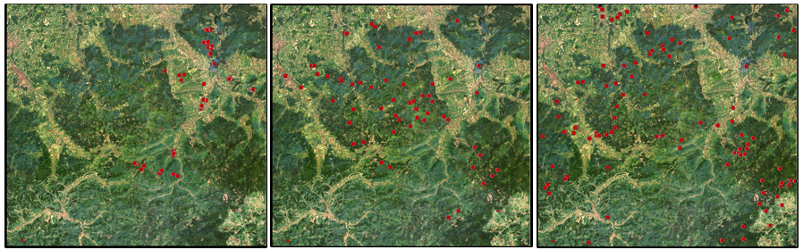
Stratify your samples - spatially, spectrally (and temporally) Your study area is likely to be diverse across space, i.e. different cover types and materials, diverse spectral classes within the same thematic class, but also environmental factors such as climate, topography, and soil may create a heterogenous mosaic of spectral features. Ideally, this variability is captured in your training data. A crude approach to achieve this, is to distribute your samples and not cluster them in smaller subregions. The image below shows the spatial distribution of three training datasets collected for forest type mapping. Notice that some training points cluster in a subset of the study region while others are well distributed.

Now how could the above theory on training data collection be translated into practise for our case study?

Exercise 2
Open the Sentinel-2 image and the previously saved .gpkg vector file in QGIS.

Identifying a suitable reference pixel. Consider the six main land cover classes (built-up, grass, broadleafed, coniferous, cropland, water) and think about a few subclasses (built-up > asphalt, concrete, roof tiles, …) for which you could select references. The latter refers to sampling the spectral classes which together make up your thematic class. Keep the above theory in mind and stratify your samples across the study area. Use very-high-resolution (VHR) background imagery from Google/ESRI in QGIS and verify the determined land cover using Google Earth. You can install a plugin in QGIS called “Send2GE” (Plugins > All > Search “Send2GE” > Install). If you select the red arrow, you will be automatically navigated to the selected location in Google Earth. This allows you to make use of the historical imagery tool. Remember that the data from Sentinel-2 is from 2019.

Be aware of the spatial resolution. The Sentinel-2 data comes with 10m spatial resolution. Accordingly, most pixels are mixed pixels, i.e. they integrate the spectra from various surface materials, potentially also different land cover classes. For reference data collection we will first try to select pixels that are nearly homogenous according to our land cover definition from above.

Sampling a point. Make the vector file editable by selecting it in the Layers panel and clicking . Next place the point within the pixel you determined the land cover label for using . A window pops-up which lets you fill in the correct classID integer value as well as the subclass description if possible, e.g. “deep water”, “shallow water” (otherwise use the main classes’ name). Leave the remaining columns blank. Make sure to save your point file frequently.

Assignment

In today’s homework assignment you will…

• … sample additional spectral reference data for our target land cover classes
• … identify the position and separability of these land cover classes in the spectral feature space of Sentinel-2

Collect training data

With the above points in mind, you can now start collecting representative reference spectra for the six land cover classes. For each of the land cover classes, identify at least 5-10 reference pixels. Determine the amount of samples based on the spectral classes within the thematic classes (some land cover classes are more diverse than others, e.g. “built-up” vs. “water”).

Plot land cover spectra

Once you have gathered your reference samples, read the .gpkg into R (see Exercise 1) and create a spectral signature plot(s). Colour the lines according to their land cover class and decide for yourself how best to visualize the results (see Exercise 1, but feel free to adjust and experiment - this is a great chance to advance your R skills).

Based on the created plots, shortly interpret:

• The overall reflectance and absorption patterns of each class across the Sentinel bands
• The spectral variance and range each land cover class shows
• The difference and similarities among classes. Identify spectral regions (bands) which could be well/not-well suited for differentiating between the classes. Which classes might be more difficult to separate, which seem to be rather easily distinguishable?

Submission

• Document your answers to the questions above with bullet points and the help of your screenshots in your .Rmd document knitted to PDF.

• Knit and upload your answers/interpretations as .pdf file, and also upload your .gpkg spectral library file onto Moodle.

• General submission notes: Submission deadline is the following Monday at 10am.

Copyright © 2023 Humboldt-Universität zu Berlin. Department of Geography.