9. Accuracy assessment

Learning goals

Understand principles of accuracy assessments
Learn how validation data is generated
Get familiar with the confusion matrix and basic accuracy scores
Assess the accuracy of your Berlin land cover map

Principle of accuracy assessment

Accuracy assessment is an crucial step in any remote sensing-based classification exercise, given that classification maps always contain mis-classified pixels and, thus, classification errors. The impact of these errors depends on many factors, including

the type of input data to the classification process,
the quality of the training signatures,
the performance of the selected classification algorithm,
the complexity of the class scheme and the separability of the underlying classes.

For subsequent use of the classification map, the map accuracy and the sources of errors have to be known. In this regard, the quality of the classification map is evaluated through comparison to validation data representing the truth (also called ‘ground truth data’). The accuracy assessment aims to provide answers to the following questions:

What is the overall accuracy of the classification map?
What is the accuracy of single classes in the classification map?
Which classes are mis-classified and confused with each other?

Validation data

Availability of validation data is indispensable for assessing the accuracy of classification maps. Mostly, validation data are represented by point samples with class labels representing the truth. These are then statistically compared to the respective class labels of the classification map.

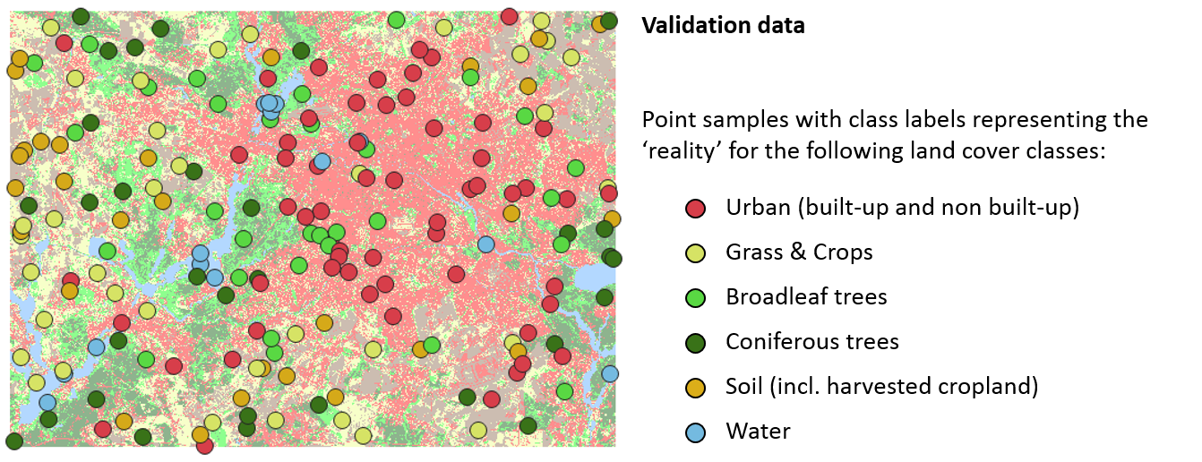
In most cases, samples are generated and labeled by the map producer. To get a statistically sound estimate of map accuracy, attention must be paid to the way sample locations are selected:

Samples should be created independently from training data
Samples should be drawn randomly (different strategies to do so, you may take a look at the advanced materials)
Samples and training data should not be autocorrelated, i.e., a minimum distance between points should be defined

Different strategies exist regarding the labeling of the samples. Often, class labels are assigned through visual interpretation of the underlying satellite image or very high resolution imagery, e.g. from Google Earth. Sometimes, samples are labeled based on field visits or based on available independent land cover information.

Confusion matrix

The example below will be used in the following to provide a step by step introduction into the basic procedure and common error metrics for assessing the accuracy of classification maps.

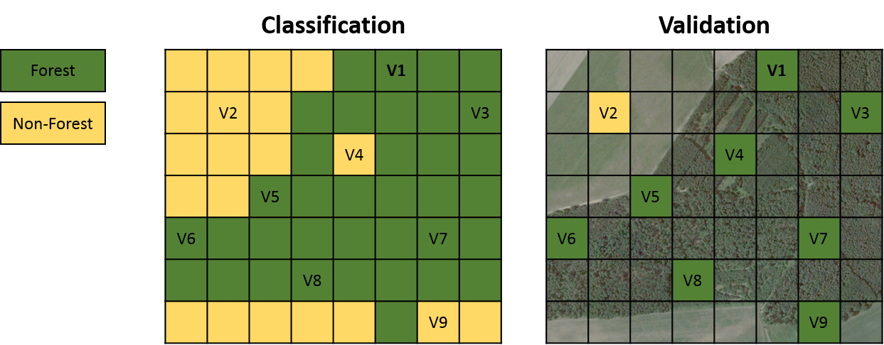
The left side illustrates a forest vs. non-forest classification result of an image with the dimension of 8 x 7 pixels. The right side illustrates a set of 9 samples with labels representing the true classes. Please note that comparison between classification and validation is mostly on a pixel-basis and samples are therefore rasterized to match with the image pixels of the classification map as demonstrated here.

From here on, we focus the further analysis on the samples by comparing predicted classes from the classification map with the true classes from the validation data.

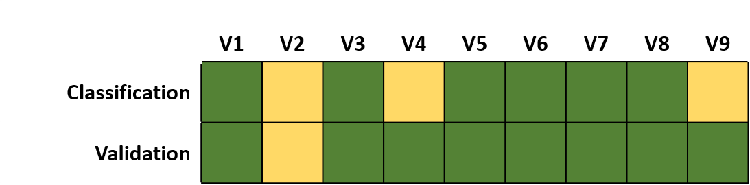
At first sight, we see both agreement but also confusion between classification and validation. A simple summary is as follows:

Classification: 
    6 x Forest samples, 3 x Non-Forest samples  
Validation: 
    8 x Forest samples, 1 x Non-Forest sample

This summary provides an indication that the classification contains errors when compared to the truth. However, it does neither provide a statistical measure on the accuracy nor information on class confusion. We therefore extend our example to identify correctly and falsely classified samples.

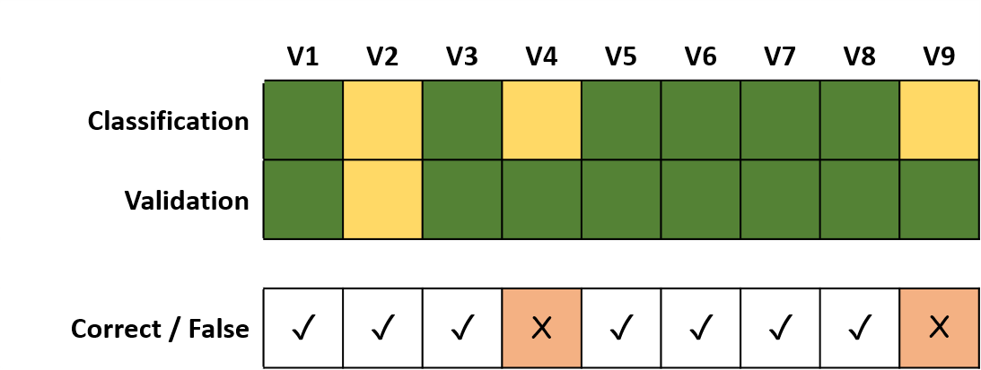
This leads to the following summary:

Correct: 
  7 out of 9 samples
False: 
  2 out of 9 samples

This summary allows us to calculate the percentage of correctly classified samples as measure of accuracy, but still does not provide information on class confusion. We therefore translate our comparison between classification and validation into a table layout, which is referred to as confusion matrix.

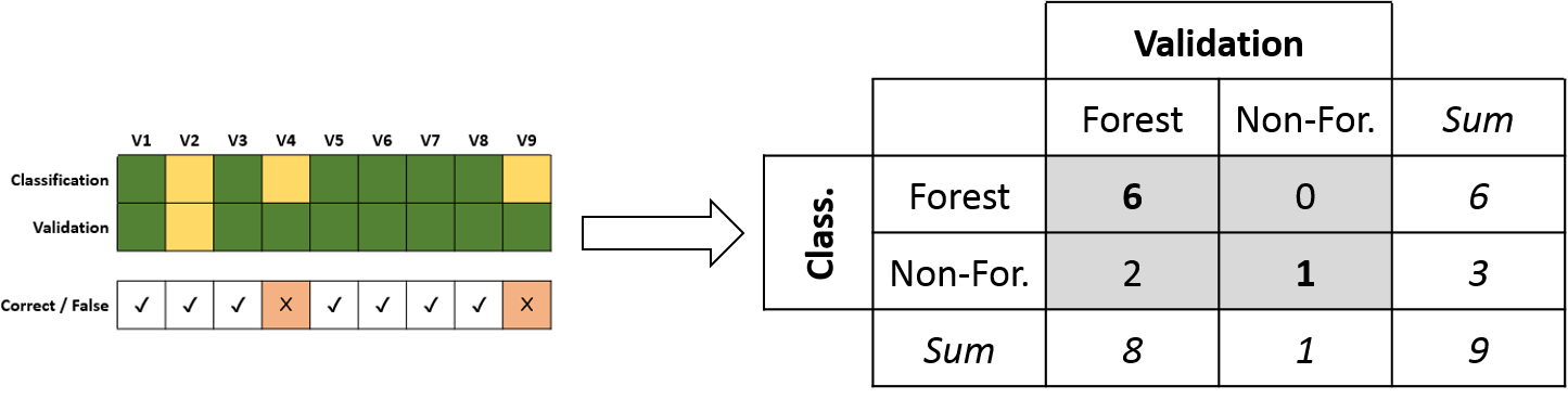
The confusion matrix is the foundation for statistical accuracy assessment and enables us to calculate a variety of accuracy metrics. The columns of the matrix contain the instances of the validation, the rows instances of the classification. The diagonal of the matrix illustrates the correctly classified samples. Row and column sums are additionally presented.

Overall Accuracy

The Overall Accuracy represents proportion of correctly classified samples. The OA is calculated by dividing the number of correctly classified samples by the total number of samples.

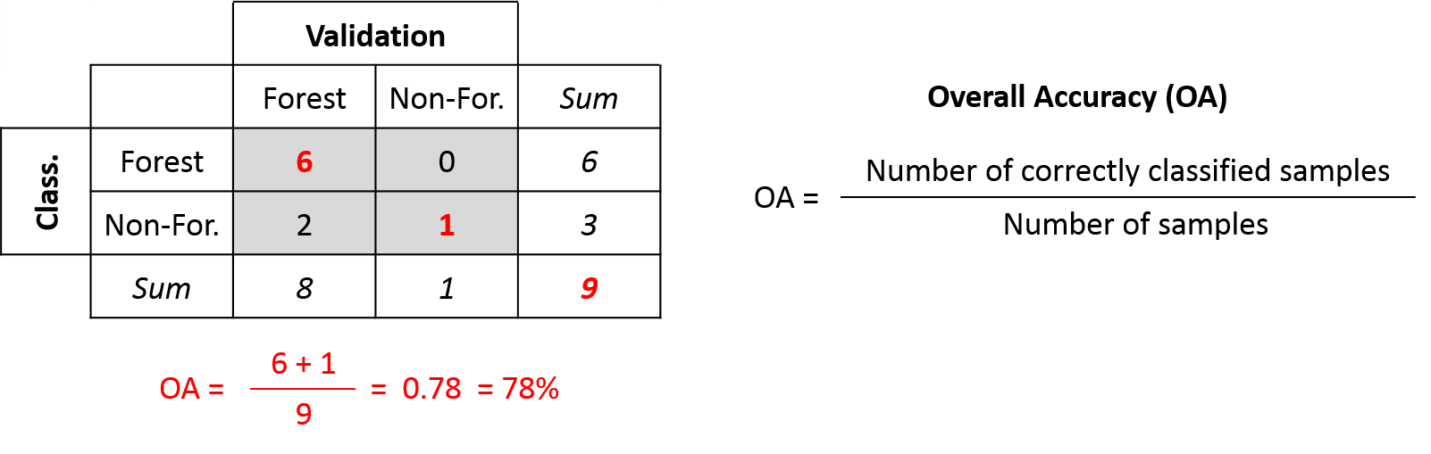
The Overall Accuracy is a general measure of map accuracy, however, does not tell us whether errors are evenly distributed for all classes. We don’t know which classes were well or poorly mapped.

User’s Accuracy & Commission Error

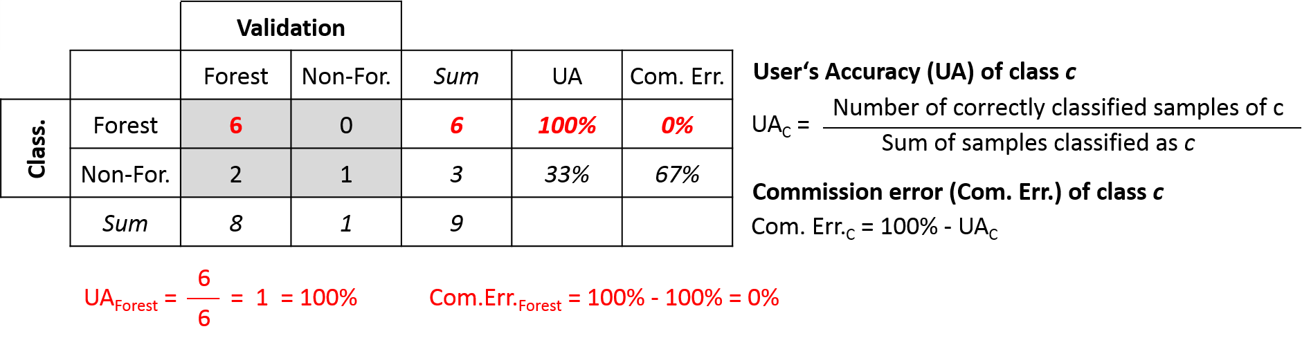
The User’s Accuracy represents class-wise accuracies from the point of view of the map user. The User’s Accuracy is calculated by dividing the number correctly classified samples of class c by the number of samples classified as class c. It therefore provides the map user with a probability that a particular map location of class c is also the same class c in truth.

The Commission Error is the complementary measure to the User’s Accuracy and can be calculated by subtracting the User’s Accuracy from 100%.

Based our initial example above, we only focus on the classification (map user perspective) and summarize the following:

User's Accuracy:
  Forest (100%): 6 correctly classified Forest samples, 6 classified Forests samples
  Non-Forest (33%):  1 correctly classified Non-Forest sample, 3 classified Non-Forests samples

Commission Error:
  Forest (0%): 0 wrongly classified Forest samples, 6 classified Forests samples
  Non-Forest (67%): 2 wrongly classified Non-Forest samples, 3 classified Non-Forests samples

The User’s Accuracy for each class is calculated by going through each row of the confusion matrix and by dividing the number of correctly classified samples through the row sum. The Commission Error is simply calculated as 100% - User’s Accuracy.

User´s Accuracy and Commission Error
A practical example: Imagine you are navigating through a desert, using a map to find an oasis. The User´s Accuracy of the class “oasis” expresses the chance, that an oasis in your map is also an oasis in reality. A low User´s Accuracy for class oasis increases your risk of walking to a falsely mapped oasis. As a complement, the Commission Error expresses the chance that you navigate to an oasis on your map but there is none in reality.

Producer’s Accuracy & Omission Error

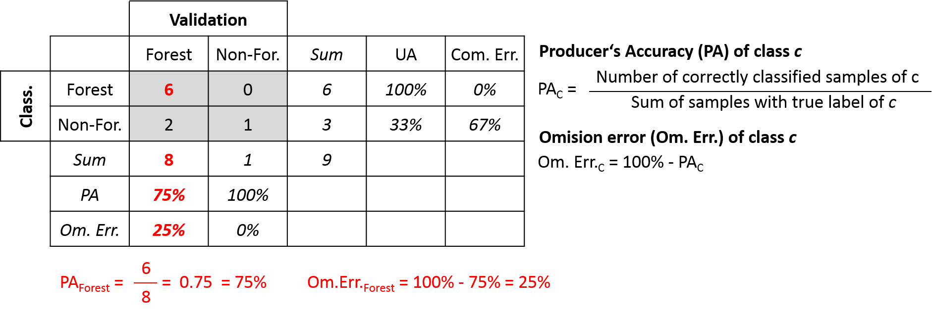
The Producer’s Accuracy represents class-wise accuracies from the point of view of the map maker. The Producer’s Accuracy is calculated by dividing the number of correctly classified samples of class c by the number of samples of with the true labels of class c. It therefore provides a probability that a particular sample of class c is mapped as the same class c in the classification map.

The Omission Error is the complementary measure to the Producer’s Accuracy and can be calculated by subtracting the Producer’s Accuracy from 100%.

Based our initial example above, we only focus on the validation (map maker perspective) and summarize the following:

Producer's Accuracy:
  Forest (75%): 6 correctly classified Forest samples, 8 Forest samples
  Non-Forest (100%): 1 correctly classified Non-Forest samples, 1 Non-Forest samples

Omission Error:
  Forest (25%): 2 wrongly classified Forest samples, 8 Forest samples
  Non-Forest (0%): 0 wrongly classified Non-Forest samples, 1 Non-Forest samples

The Producer’s Accuracy for each class is calculated by going through each column of the confusion matrix and by dividing the number of orrectly classified samples through the column sum. The Omission Error is simply calculated as 100% - Producer’s Accuracy.

Producer´s Accuracy and Omission Error
Back to the desert example: you are still looking for an oasis in the desert. The Producer´s Accuracy of the class “oasis” expresses the chance, that a real oasis is also included in your map. As a complement, the Omission Error expresses the chance that you suddenly find an oasis, which is not included in your map.

Confusion matrix in practise

The figure below illustrate an exemplary accuracy assessment from a land cover classification.

Exercise 1
Complement the confusion matrix with the following information:

Instance ‘Broadleaf forest’ vs. ‘Broadleaf forest’
Instance ‘Urban’ vs. ‘Agriculture’
Number of samples for ‘Urban’
Number of classified ‘Needleleaf’ samples

Calculate the following accuracy metrics:

Overall Accuracy
Producer’s Accuracy for the class ‘Urban’
Omission Error for the classes ‘Agriculture’ and ‘Water’
User´s Accuracy for the class ‘Urban’
Error of Commission for the classes ‘Agriculture’ and ‘Water’

Assignment

Download the session materials from our shared repository. The materials contain a validation point layer for the 2019 land cover of Berlin.

The goal of this assignment is to conduct an accuracy assessment of your final land cover classification of Berlin. The provided validation data shapefile comprises 145 independently drawn sample points which were labeled through visual interpretation of dense Landsat-Sentinel-2 time-series in combination very-high-resolution Google Earth imagery.

1) Extend reference data and combine validation layers

We have done most of the work for you and labeled 145 samples. Your task is to extend this dataset and thereby learning how such a sample should be generated.

You do this by generating a random stratified sample based on your classification map. For each class (= stratum), you sample \(n\) samples randomly across the image.

classification  # your land cover map from last session
stratified_sample <- terra::spatSample(classification, size=3, 
                                        method="stratified", na.rm=TRUE, 
                                        as.points=TRUE, values=FALSE)

# add the new points to existing validation layer
validation <- vect("../../LC_BERLIN_2019_VALIDATION.gpkg")
validation <- rbind(validation, stratified_sample)

# write to disc
writeVector()

Open the extended point layer and QGIS, and just like in Session 5, label the 18 new points accoridng to their true land cover. Do not take a look at the land cover map, just interpret the Sentinel-2 imagery and Google Earth History images.

2) Create confusion matrix

# extract predicted (pred) land cover with observed (obs) validation points
df_pred_obs <- data.frame(
  terra::extract(classification, validation, bind=T)
)

# remove any no data values
df_pred_obs <- na.omit(df_pred_obs)

# 'class' is the predicted land cover columns
# 'classID' is your validation land cover column

# create confusion matrix
predobs <- table(df_pred_obs[c('class', 'classID')])
install.packages("caret")
library(caret) 
confusionMatrix(predobs, mode = "prec_recall")

3) Interpret accuracy assessment report

The accuracy assessment report comprises different accuracy metrics that go beyond the introduced measures. Please focus on the following information:

Confusion matrix
Overall Accuracy
User’s Accuracy & Omission Error per class (generally termed “Precision”)
Producer’s Accuracy & Omission Error per class (generally termed “Recall”)

Interpret the accuracy assessment report with regard to the following questions:

What is the Overall Accuracy of your map?
Which classes were well, which were poorly classified?
Which classes were most confused with each other?
Which classes tend to be overestimated, which underestimated in your land cover map? (Commission vs. Omission)

4) Discuss map error sources

Visualize your classification map and and the Sentinel-2 image and/or very high resolution Google Earth imagery in QGIS.
Search for 2 different example locations, which illustrate mis-classified surfaces according to the confusion you observed in the accuracy assessment.
Discuss the potential error source for each location.
Search for 2 different example locations, which illustrate well-classified surfaces according to the confusion you observed in the accuracy assessment.
Discuss why these pixels could accurately be predicted

Portfolio Readings
Preparation for Portfolio: Reading 4 primary research articles until 10th Jan 2024. Description and articles on Moodle (Session: Accuracy Assessment).