Probability

Probability describes of how likely it is that an event \(a\) occurs, given all possible events \(A\):

\(P(a) = \frac{\text{Count of a}}{\text{Count of A}}\)

Example: The probability of getting a six when rolling a dice once is \(P(6) = 1/6\).

We can also calculate the probability that event \(a\) or event \(b\) will occur, given they are mutually exclusive, by adding their individual probabilities:

\(P(a \cup b) = P(a) + P(b)\)

Example: The probability of getting a six or a three when rolling a dice once is \(P(6 \cup 3) = P(6) + (6) = 1/6 + 1/6 = 1/3\)

When we are interested in the joint probability that event \(a\) and \(b\) occurs at the same time, given the events are independent, we calculate the probability by multiplying the individual probabilities:

\(P(a \cap b) = P(a) * P(b)\)

Example: The probability of getting two times a six when rolling a dice two times is \(P(6 \cap 6) = P(6) * P(6) = 1/6 * 1/6 = 1/36\)

Conditional probabilities

Assume we have an urn with 30 balls in it. Of the 30 balls, 10 are wooden and 20 are made out of plastic. From the 20 balls made out of plastic, 8 are of red color and 12 are of blue color. From the wooden balls, 4 are of red color and 6 are of blue color.

What is the probability of drawing …

a red ball \(P(R)\)
a wooden ball \(P(W)\)

Moreover, what is the probability of drawing…

a red, wooden ball: \(P(W \cap R)\)
a blue ball made out of plastic \(P(P \cap B)\)

Contingency-table

We can easily represent all possible events in a contingency-table:

	Red	Blue	Sum
Wood	4	6	10
Plastic	8	12	20
Sum	12	18	30

The probabilities of each event are:

	Red	Blue	Sum
Wood	\(P(R \cap W)=\frac{4}{30}\)	\(P(B \cap W)=\frac{6}{30}\)	\(P(W)=\frac{10}{30}\)
Plastic	\(P(R \cap P)=\frac{8}{30}\)	\(P(B \cap P)=\frac{12}{30}\)	\(P(P)=\frac{20}{30}\)
Sum	\(P(R)=\frac{12}{30}\)	\(P(B)=\frac{18}{30}\)

While drawing a ball from the urn, we already feel that the ball is made of wood. What is the probability that it is red in color? Easy to calculate using the rule of conditional probabilities:

\(P(R|W) = \frac{P(R \cap W)}{P(W)} = \frac{\frac{4}{30}}{\frac{1}{3}} = 0.4\)

Observations

Random variables

A random variable is a variable that can take on a set of possible values, each with a distinct probability.

Example: The random variable ‘age’ can take any value between 0 and \(\infty\), though picking a random person, it is more likely she is 35 than 110.

Sample

Simply speaking, a sample consists of a set of realisations of a random variable. The size of a sample is termed \(n\).

Example: If I pick one person (\(n = 1\)) in this class, a realisation of the random variable ‘age’ might be \(S = \{26\}\). If I pick three persons (\(n = 3\)), the realizations might be \(S = \{22, 28, 32\}\).

Sampling

Drawing a sample from a population requires a defined procedure:

Simple random sampling
Systematic sampling
Stratified sampling
Clustered sampling

All those procedures have in common that each data point has a well-defined probability of being included in the sample. We then speak of a probability sampling design. There are also non-probability sampling designs.

Pinewood data

Suppose, we randomly selected 150 trees in the fictitious land of Pinewood. Our sample then has size \(n\)=150. The sampling units are trees. And for each tree (sampling unit) we collect some data/variables. For example, for each tree we measured the diameter at breast height (DBH) in cm.

Descriptive statistics

Descriptive statistics summarize the characteristics of a dataset like the central location around which the majority of the observations cluster (e.g., mean and median) and the spread of the observations (e.g., variance and standard deviation). Below are the summary statistics of the Pinewood tree sample (Table 1).

Table 1: Descriptive statistics of the tree dataset.
Statistic	Value
Mean	56.5
Median	57.0
Mode	67.0
Variance	255.4
Standard deviation	16.0
Coefficient of variation	0.3
Interquartile range	21.0
Skewness	0.1
Kurtosis	2.6

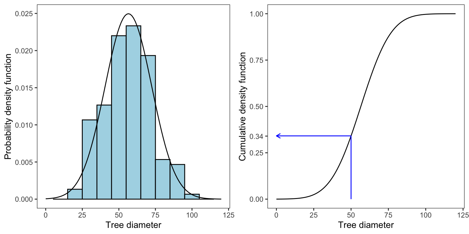
We can inspect the distribution of tree DBH in Pinewood by means of a histogram (Fig. 1). When drawing a histogram the choice of binning can have a substantial effect on the resulting visualization. There are a number of formulas for estimating meaningful width or number of bins. For example, the number of bins \(k\) might be determined with the Sturge’s rule: \(k=1+log_{2}(n=150) = 9\).

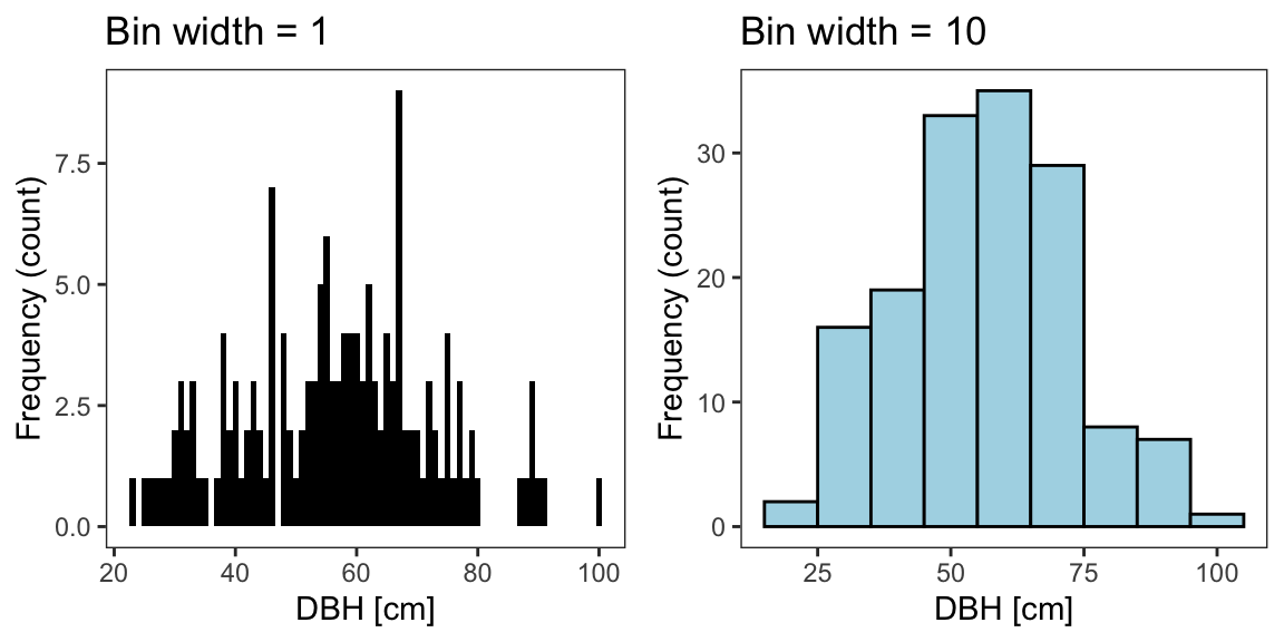
Fig. 1 Frequency distribution of trees collected in Pinewood forest.

From frequency to probability

The frequency distribution of the tree sample tells us which DBH classes are more frequent and which are rare. The DBH classes are here represented by the bins in the histogram (Fig. 1). If we added a new tree to our sample, it is more likely that it falls in the frequent DBH classes (bins) than in the rare classes. Thus, we can infer from the frequency distribution of the sample the probability that a tree in Pinewood has a certain DBH value. The notion that we infer from the frequency distribution of a sample the probability of an outcome/event in the underlying population is the basis of a many statistical methods.

Statistical inference is the process of using a sample to infer the properties of a population.

Figure 2 below shows a histogram of the absolute frequency (left) and the relative frequency (middle). We can use the relative frequency (proportions) to estimate the probability of a random tree in the Pinewood forest (the population) to fall into that bin, i.e., the diameter range described by that bin. The tallest bin has 35 observations (out of 150). So, the proportion of trees in that bin is \(0.23\) (\(\frac{35}{150}\)). Hence, we estimate the probability that a tree is in that bin’s diameter range to be 0.23.

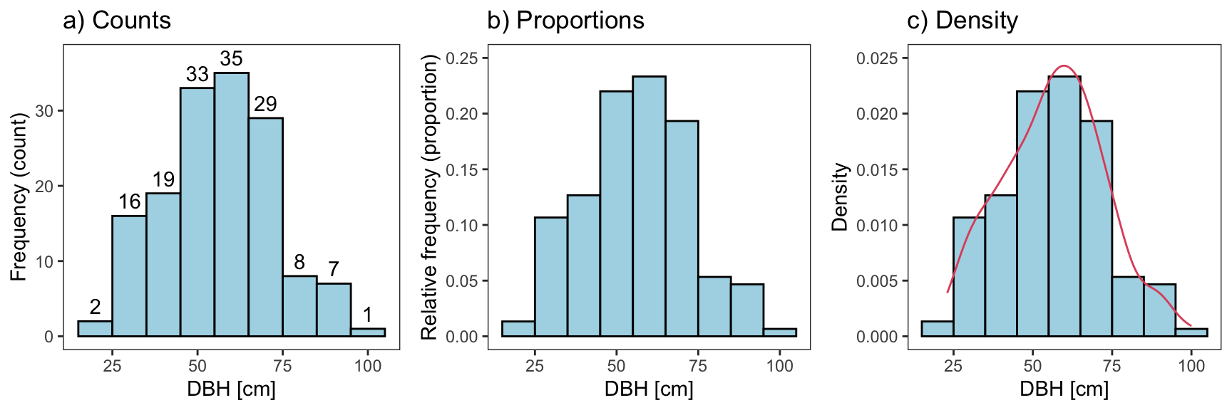
Figure 2. Frequency, proportions, and density distribution of trees.

The histogram is an effective tool for visualizing distributions of samples but too crude for estimating probabilities. A better way for estimating the probability distribution of a population is provided by the concept of density. The density concept describes the probability distribution of a population as a continuous function: the probability density function (pdf). Since there are an infinite number of real numbers infinitely close on that function, we cannot estimate the probability of a single point \(x\) falling onto that function. That value would be zero, i.e., \(P(X=x)=0\). However, we can estimate the probability that \(x\) falls into a tiny region around \(x\).

To illustrate the density concept, we can turn our frequency histogram into a density histogram (Figure 2). Recall that the tree proportion of the tallest bin was \(0.23\). Since the width of the bin is 10 \(cm\), the density is \(0.023\). Conversely, the area in that bin is \(0.023 \times 10 =0.23\). The area under the density function described by an interval \((a,b)\) is the probability that a tree \(x\) falls into that interval: \(P(a < X < b)\). Thus, the area under the entire curve sums to 1.

The density histogram is illustrative but it is still crude and blocky. For continuous variables, we’d expect a smoother probability distribution function (at least for large populations). The histogram is crude, because it is based on a comparably small sample which may not include all values of the population. For example, we did not measure a tree with a DBH of 24 and 83, but it is likely that such trees exist in the population. A smoother density estimate can be obtained using kernel density methods (red line, Figure 2). But, typically we use well-known probability distributions to estimate the density distribution of a population.

Probability distributions

Probability distributions describe the likelihood of a random variable taking a certain value. Probability distributions have the following characteristics:

They are described through a probability density function (pdf)
The pdf has a set of parameters describing its location and variance
The integral between \(a\) and \(b\) is the probability that values between \(a\) and \(b\) occur
The complete area below the pdf is 1
All values of the pdf are independent
The pdf can be expressed as cumulative distribution function (cdf)

The most important distributions are:

Normal distribution
Binomial distribution
Poisson distribution
Log-normal distribution
t-distribution
F-distribution

Though there are many more used in our field…

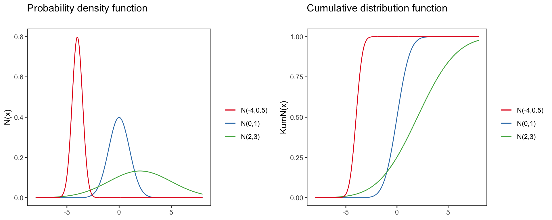
Normal distribution

\(\begin{aligned} N(x) = P(X=x \vert \mu, \sigma) = \frac{1}{\sigma \sqrt{2\pi}}e^{\frac{-(x-\mu)^2}{2*\sigma^2}} \end{aligned}\)

Parameter of the normal distribution:

Domain: \(x \in \mathbb{R} = (- \infty,\infty)\)
Mean: \(\mu\)
Variance: \(\sigma^2\)

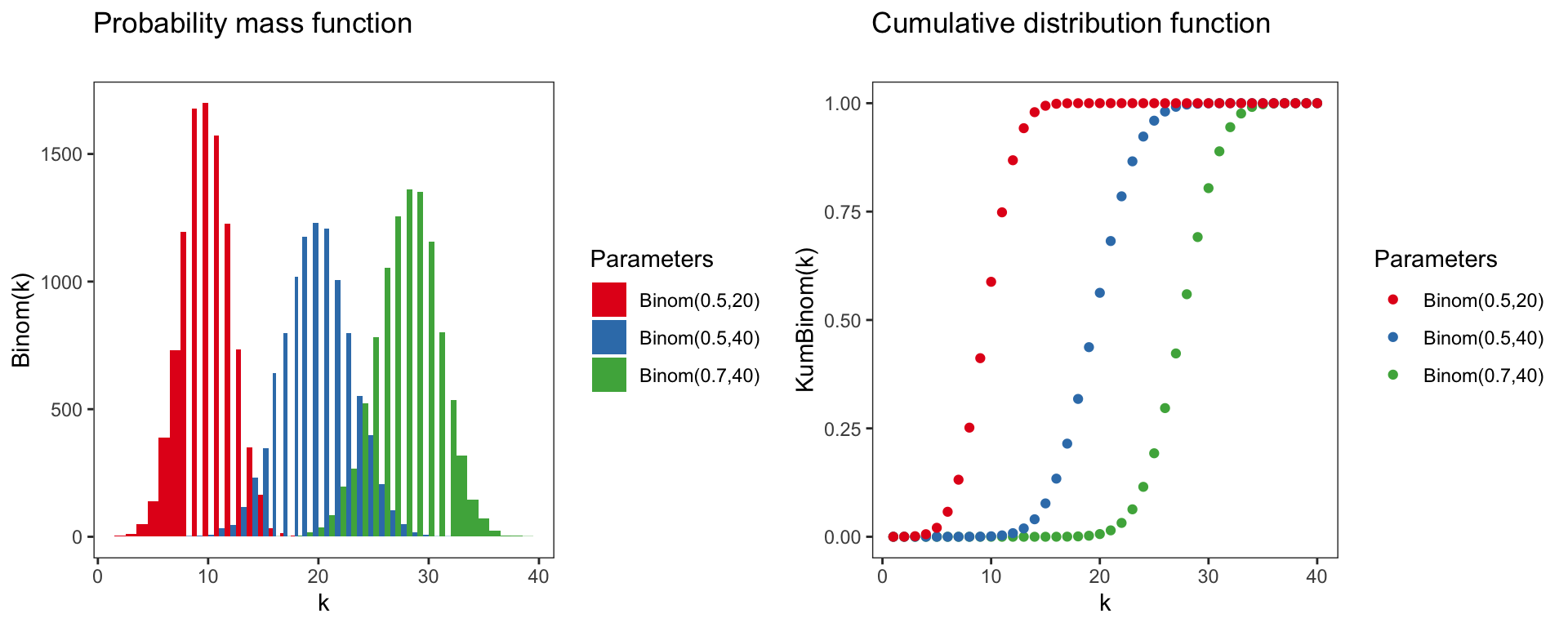
Binomial distribution

\(\begin{aligned} Binom(k) = (X=k \mid p,n) = \begin{pmatrix} n \\ k \end{pmatrix} p^{k}(1-p)^{n-k} \end{aligned}\)

Parameter of the binomial distribution:

Domain: \(k \in \mathbb{N}_{0} = \{0,1,2,3,...\}\)
Mean: \(np\)
Variance: \(np(1-p)\)

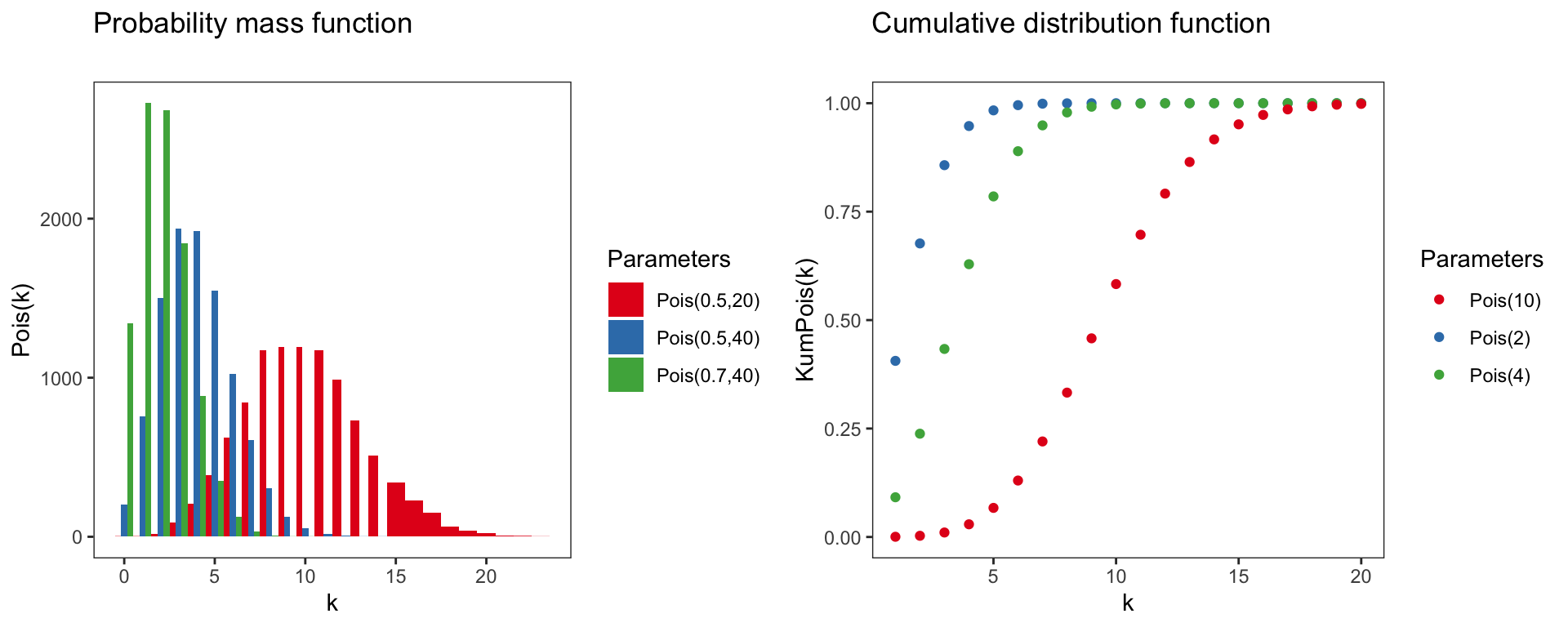
Poisson distribution

\(\begin{aligned} Pois(k) = P(X=k \mid \lambda) = \frac{\lambda^{k}e^{-\lambda}}{k!} \end{aligned}\)

Parameter of the poisson distribution:

Domain: \(k \in \mathbb{N}_{0} = \{0,1,2,3,...\}\)
Mean: \(\lambda\)
Variance: \(\lambda\)

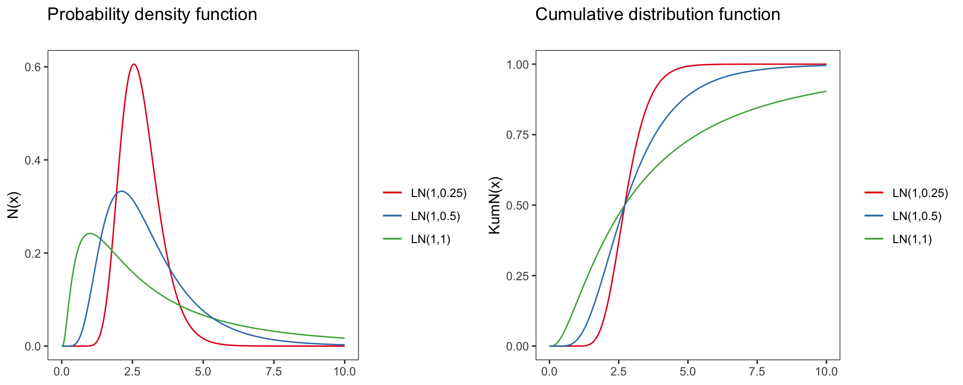
Log-normal distribution

\(\begin{aligned} logN(x) = P(X=x \vert \mu, \sigma) = \frac{1}{x \sigma \sqrt{2\pi}}e^{-\frac{(ln x-\mu)^2}{2*\sigma^2}}, x>0 \end{aligned}\)

Parameter of the log-normal distribution:

Domain: \(x \in \mathbb{R}_{0}^{+} = (0,\infty)\)
Mean: \(e^{2\mu+sigma^{2}/2}\)
Variance: \((e^{\sigma^{2}-1})e^{2\mu+sigma^{2}}\)

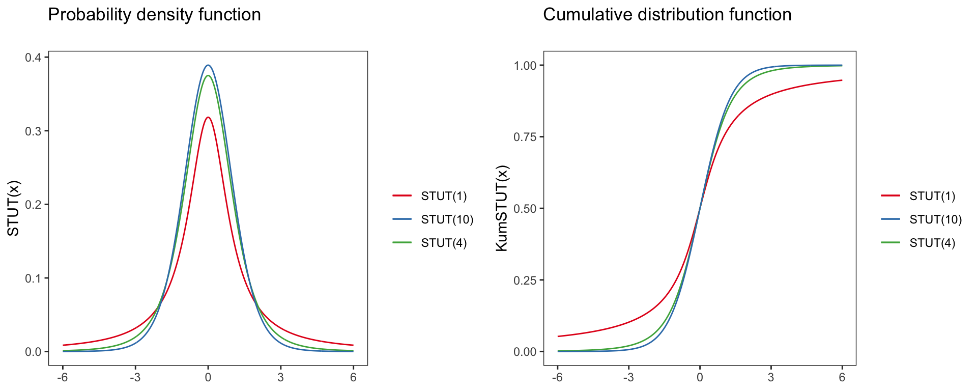
t-distribution

\(\begin{aligned} STUT(x) = (X=x \mid v) = \frac{B(\frac{v+1}{2})}{\sqrt{v*\pi}B(\frac{v}{2})}(1+\frac{x^{2}}{v})^{-\frac{v+1}{2}} \end{aligned}\)

With \(B(x,y)\) being the Euler Beta-function.

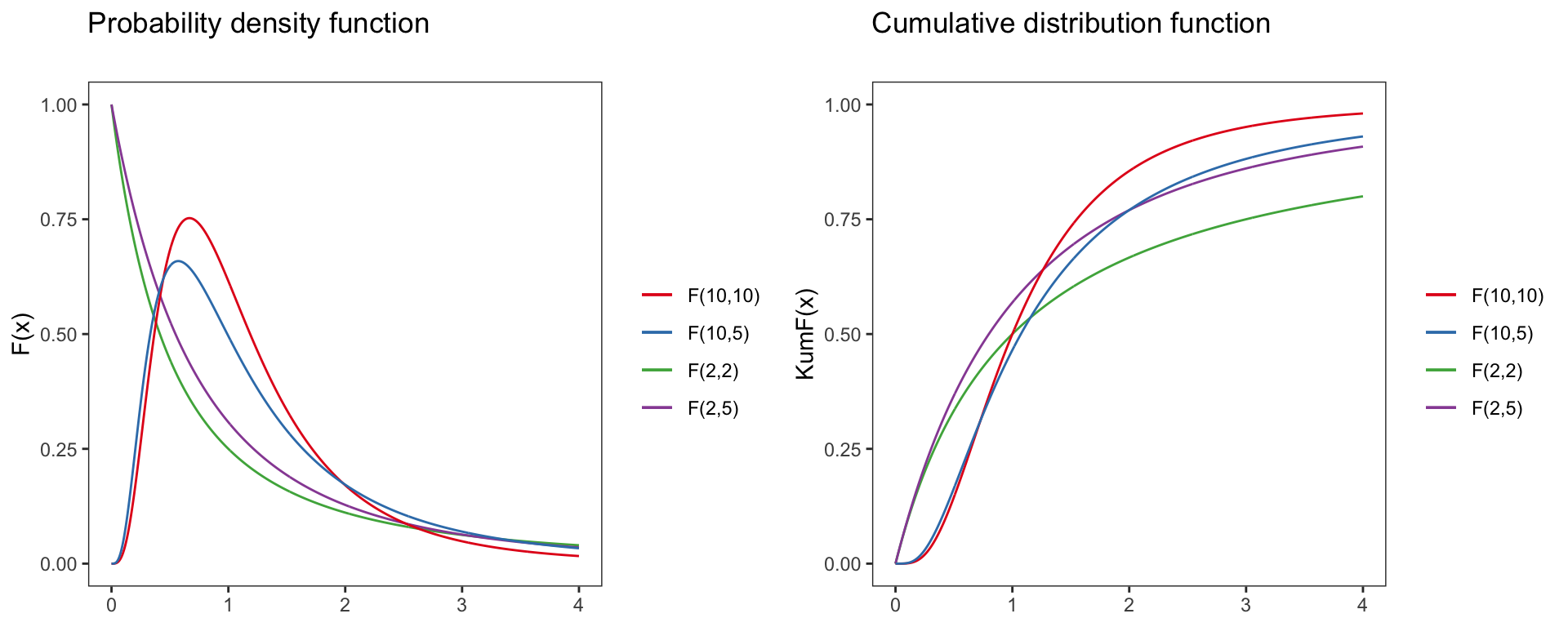
F-distribution

\(\begin{aligned} F(x) = (X=x \mid v_{sp1}, v_{sp2}) = \sqrt{\frac{(v_{sp1}x)^{v_{sp1}} v_{sp2}^{v_{sp2}}}{(v_{sp1}x+v_{sp2})^{v_{sp1}+v_{sp2}}}} \div {xB(\frac{v_{sp1}}{2},\frac{v_{sp2}}{2})} \end{aligned}\)

Density estimation

Commonly, we use one of the known parametric distributions to estimate the probability distribution of a population. We do not know the true probability distribution function (\(pdf\)) of the population. We can only make an educated guess by inspecting histograms of the sample and based on experience. We must also keep in mind that \(pdf\)’s are models with which we describe populations. They are not intrinsic properties of populations. We may assume a population can be described with a normal distribution, but it is not a physical explanation.

Once we selected a distribution, we need to find the parameters of that distribution. We do not know the parameters, but we might estimate them from our sample. For example, assuming a process is normally distributed, we can estimate the parameter \(\mu\) and \(\sigma\) from the sample, i.e., be substituting \(\mu\) with the sample mean and \(\sigma\) with the sample standard deviation.

Going back to Pinewood, the normal distribution seems an appropriate choice to describe the diameter distribution. The estimated parameters (denoted by the hat symbol ^) are taken from the sample mean and standard deviation:

\[\hat{\mu} = \overline{x} = 56.5\]

\[\hat{\sigma} = s = 16\]

We can plot the estimated normal \(pdf\) on top of the sample distribution, and we can also plot the cumulative density function (\(cdf\)). We can then grab from the \(cdf\), the probability that a tree has a DBH of up to \(x\), i.e., \(P(X\leq x)\). For example, there is a 0.34 probability that a tree in Pinewood is less than or equal to 50 cm.

Sampling distribution

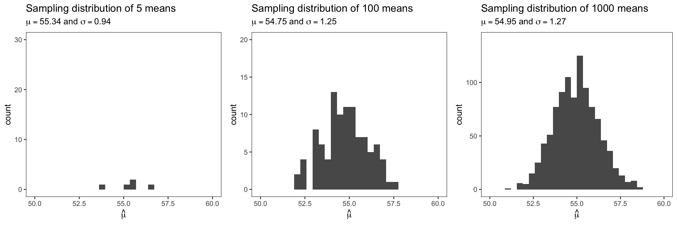
We just used a sample (of trees) to estimate the parameters \(\hat{\mu}\) and \(\hat{\sigma}\) of the probability density distribution of the tree population in Pinewood. Since a sample usually represents a fraction of the population, our estimates have uncertainties associated with them. We can illustrate this using the following theoretical construct: If we repeated the sampling, we would obtain a different estimate every time we collected a new sample. Let’s assume we repeatedly sampled 150 trees 5 times, 100 times, and 1000 times, respectively. We would get 5, 100, and 1000 sample means, respectively. The next figure shows the distribution of these sample means (NOT the distribution of individual trees). Such a distribution is called the sampling distribution (of the mean diameter). The more often we repeat the sampling the more closely the distribution of the means resembles a normal distribution (Central Limit Theorem). Hence, we can describe the sampling distribution itself with a normal distribution, with a mean and a standard deviation.

A sampling distribution is a probability distribution of a statistic that is obtained through repeated sampling of a specific population.

Usually, we do not and cannot repeat sampling. Then, why all this? The sampling distribution is an important concept that we can use to test if an estimated parameter is significantly different from some other expected value. The sampling distribution recognizes that there is in fact a range of possible outcomes for a parameter. In other words, the precision of our estimate is nonzero.

Sampling variance

Concept

The sampling variance (or standard deviation) of a sample-based estimate describes the precision of that estimate. For the Pinewood forest, the mean and standard deviation of the sampling distribution of the mean was \(\bar{\hat{\mu}}=\) 54.95 and \(\sigma_{\hat{\mu}}=\) 1.27, respectively (see above figure with 1000 repeated samples). Recall with a normal distribution, ~68% and ~95% of the observations fall within 1 and 2 standard deviations, respectively. Hence, we can say that our estimate of mean DBH falls into the range of 54.95 \(\pm\) (2 \(\times\) 1.27) cm 95% of the times (if we repeated the sampling). Or 95% of the times the mean DBH is between 52.41 and 57.49cm.

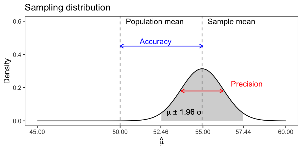
It is important to understand that we do not know the location of the true parameter, here the population mean. So, we cannot say how close our estimate is to the true value. We can say that our estimate is within a range of estimates that we would obtain if we would repeat the sampling. A precise estimate with a low sampling variance is not necessarily an accurate estimate. If the sample is biased, the true mean may lie outside the sampling distribution. Typically, we can reduce or eliminate bias through the choice of sampling and the choice of estimators. In Pinewood, we employed random sampling, and the sample mean is an unbiased estimator of the population mean, if the underlying population follows a normal distribution.

Standard error

The standard error (\(SE\)) of a statistic (usually an estimate of a parameter) is the standard deviation of its sampling distribution or an estimate of that standard deviation. For the fictitious Pinewood forest, we already estimated the standard error by sampling the forest repeatedly 1000 times (\(SE=\sigma_{\hat{\mu}}=\) 1.27).

In practice, repeated sampling is not an option. However, the variation in sampling means is linked to the (population) variance and the sample size. So, usually, we infer the SE from the sample variance (standard deviation) and sample size using the following formula:

\(SE = \frac{s}{\sqrt{n}}\)

where \(s\) denotes the standard deviation of the tree sample (not! the sampling distribution) and \(n\) denotes the sample size. Plugging in the corresponding values of the Pinewood sample, we get:

\(SE = \frac{15.98}{\sqrt{150}} = 1.3\)

…which is pretty close to our previous SE estimate of 1.27 from repeated sampling. Note, increasing sample size increases precision, independent of the population size!

Confidence interval

The confidence interval (CI) provides a means to obtain a range of possible estimates based on a specified level of confidence. Note, the confidence interval does not describe the variability in the unknown parameter. Rather, it reflects the amount of random error in the sample. More specifically, a 95% confidence interval means, if we were to take 100 different samples and compute a 95% confidence interval for each sample, then approximately 95 of the 100 confidence intervals contain the true mean value (\(\mu\)).

In practice, we select one random sample and generate one confidence interval, which may or may not contain the true mean. We cannot say that the population mean has a 95% probability of being included in this one interval. We can say that we are 95% confident that our interval includes the population mean. The former (false) statement implies that the confidence interval is fixed and the population mean is variable. In fact, it is the other way around: the unknown population parameter is fixed and the confidence interval expresses uncertainty in the interval due to sampling.

The theoretical sampling distribution of the parameter is normally distributed (following the central limit theorem). This allows us to use a standard normal distribution to estimate the range of sample means included in the central 95% of all sampling means:

\(CI_{95\%} = \overline{x} \pm SE * Z\)

with:

\(Z = \Phi^{-1}(0.975) = 1.96\) and \(\Phi \sim N(0, 1)\).

The quantile itself is often written \(\phi^{-1}(0.975)\), where \(\phi\) is standard notation for the cumulative distribution function of the normal distribution.

For our example, the 95% confidence interval is:

\(CI_{95\%} = 1.96 \times \frac{15.98}{\sqrt{150}} = 2.56\)

Hence, we estimated that trees in Pinewood have a mean DBH of 56.5 cm with a 95% CI ranging between 54 and 59.1cm.

Null hypothesis significance testing

Comparing samples

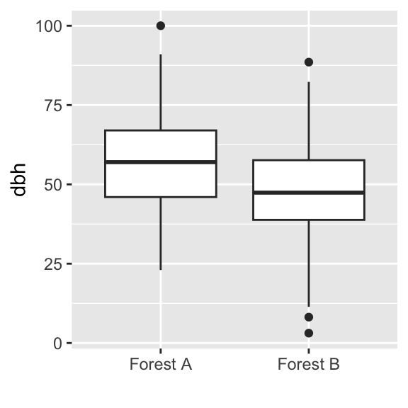
Suppose we have sampled another 150 trees in another forest. We can compare both samples using boxplots.

Null hypothesis

We might ask following question: Are the mean DBH values the same among both forests?

To test this, we formulate a precise null hypothesis \(H_{0}\): The mean DBH is equal among both samples, that is \(\overline{x}_{sp1} = \overline{x}_{sp2}\)

The principal idea behind NHST is to test how likely it would be to draw our sample at hand, assuming that \(H_{0}\) is true. Hence, we want to know \(P(D|H_{0})\). If \(P(D|H_{0})\) is very small, we might safely reject \(H_{0}\).

t-test

The NHST for two means is called a t-test (or Student’s t-test). The basic idea behind the t-test is that the difference between two sample means would be exact zero if they were the same. Hence, under the assumption of \(H_{0}\), a large difference is very unlikely. The t-test assumes that the samples are normally distributed and that the variances of the two samples are equal.

As measure of difference in sample means, which also incorporates the standard deviation, we make use of the empirical t-value:

\(t = \sqrt{\frac{n_{sp1}*n_{sp2}}{n_{sp1}+n_{sp2}}}*\frac{\overline{x}_{sp1}-\overline{x}_{sp2}}{S}\)

with \(\overline{x}\) being the sample means, \(n\) the sample size, and \(S\) the weighted paired standard deviation defined as:

\(S = \frac{(n_{sp1}-1)*s_{sp1}^{2}+(n_{sp2}-1)*s_{sp2}^{2}}{n_{sp1}+n_{sp2}-2}\)

The probability that the empirical t-value deviates from zero, given \(H_{0}\) is true, is described by a t-distribution, which has only one parameter, the degree of freedom: \(v=n_{sp1}+n_{sp2}-2\).

Lets calculate the t-value, degrees of freedom, and p-value for our example:

The sample means were 55.5 cm and 49.3 cm, respectively. Entering both in the equation for the t-value yields \(t = 3.6\), with 298 degrees of freedom. Subtracting the area between \([-t;+t]\) of the t-distribution from one yields \(p=0.0004\).

Hence, the difference in means we observed in our samples is very unlikely under the assumption of \(H_{0}\) being true. We thus might safely reject \(H_{0}\) and conclude that the mean DBH values are significantly different between both samples.

F-Test

The F-test aims at testing the difference in the variances between two samples. Like the t-test, the F-test assumes that the samples are normally distributed. The null hypothesis \(H_{0}\) is: The sample variances are equal \(s^{2}_{1} = s^{2}_{2}\).

The test statistic is the F-value, calculated as the ratio of the sample variances:

\(F = \frac{s_{sp2}^{2}}{s_{sp1}^{2}}\).

Assuming that \(H_{0}\) is true, the F-value follows the F-distribution with two parameters:

\(v_{sp1}=n_{sp1}-1\) and \(v_{sp2}=n_{sp2}-1\).

The sample variances in our example were 15.7 and 14.3, respectively. The empirical F-values is 0.91, with 149 degrees of freedom for both samples. Subtracting the area between \([-F;+F]\) of the F-distribution from one yields \(p=0.72\).

This results indicates that there is a high probability of obtaining a variance ratio similar to ours under \(H_{0}\). We thus cannot safely reject \(H_{0}\) and conclude that the variances are not significantly different.

p-value

The p-value is the most loved and hated value in science. Whole scientific disciplines build upon the p-value in drawing their conclusions from data, most often taking an arbitrary threshold of \(p<0.05\) as indication to reject \(H_{0}\).

Even though the p-value has a clear definition (\(P(D|H_{0})\)), it is very often misinterpreted. Here are the common pitfalls:

The p-value does NOT tell you anything about the probability of the hypothesis given your data (\(P(H_{0}|D)\))
The p-value is not a measure of effect size, that is it does NOT tell you anything about the strength of a difference
There is NO mathematical proof behind thresholds indicating significance (such as \(p<0.05\))
A smaller p-value is NO indication that a difference is more important than one with a larger p-value

I you’re interested in the abuse of p-values, please see: http://www.nature.com/news/statisticians-issue-warning-over-misuse-of-p-values-1.19503

Example of p-value misuse:

We sampled Nitrate concentrations in two catchments:

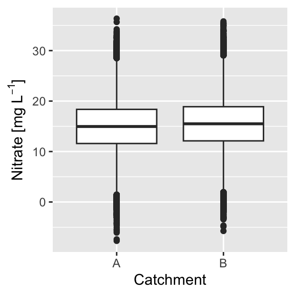
Both sampels are taken from intensive measurement sites, with n = 100,000 and a sampling error of 0.3 \(mg L^{-1}\). Do you think the difference in Nitrate concentration is substantial?

Calculating the p-value we get \(p < 0.000001\), indicating a highly significant difference. The difference in means, however, is only 0.5 \(mg L^{-1}\), which is close to the measurement error.

Correlation

Scatterplots

With our first sample, we also measured tree height:

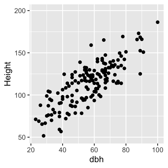
To quantify the strength of the relationship between DBH and height we make use of correlation analysis.

Correlation coefficient

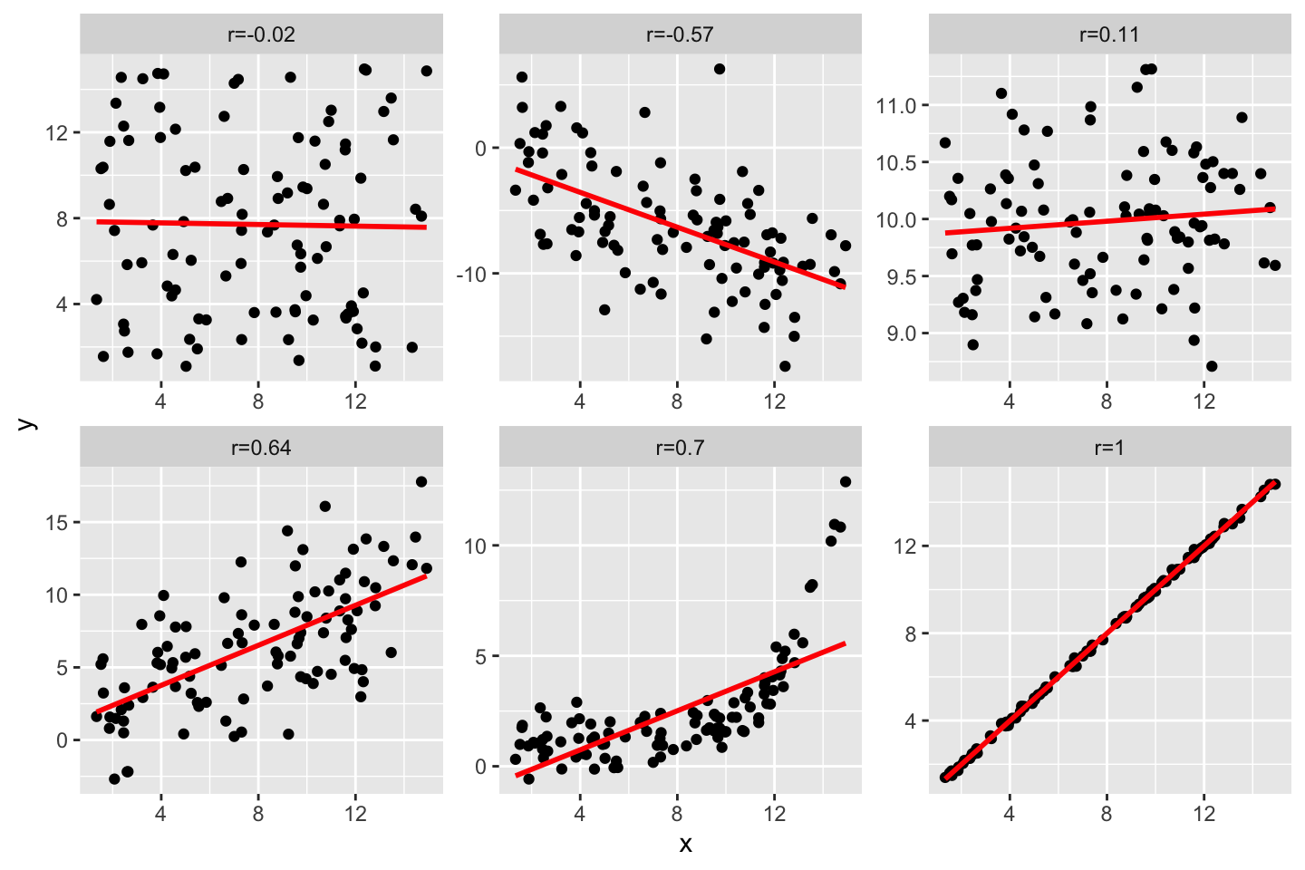
The most commonly used correlation coefficient, the Pearson correlation coefficient, is defined as:

\(r_{xy} = \frac{Cov(x,y)}{\sigma(x) \sigma(y)} = \frac{\frac{1}{n}\sum_{i=1}^{n}(x_{i}-\overline{x})(y_{i}-\overline{y})}{\sqrt{\frac{1}{n} \sum_{i=1}^{n}(x_{i}-\overline{x})^2}*\sqrt{\frac{1}{n}\sum_{i=1}^{n}(y_{i}-\overline{y})^2}}\)

and measures the linear monotonic increase in X when Y increases (or the other way round). It ranges from -1 to +1, where -1 indicates a perfect negative correlation, values close to zero indicate weak correlation, and +1 indicates perfect positive correlation.

Calculating the Pearson correlation coefficient for our examples yields \(r_{xy}=0.8\), which indicates a strong positive relationship between DBH and height.

For ordinal data or for data that are not normally distributed there exist alternative correlation coefficients, in particular the Spearman rank-correlation coefficients and Kendall’s Tau.