- Bayes rule
- Useful syntax
7. Introduction to Bayesian inference
Humboldt-Universität zu Berlin | Geography Department
Bayes rule
This week, we will apply Bayes rule to a simple exercise, which will be introduced in class. Below you find useful R syntax that will help you code the exercise.
Bayes rule (in discrete form) is:
Pr
\Pr(H_j|D) is the posterior probability, i.e. the probability of hypothesis H_j given the data (evidence) D at hand.
\Pr(H_j) is the prior probability, i.e. the probability of hypothesis H_j before we have seen (unconditional on) any data.
\Pr(D|H_j) is the likelihood of data D given hypothesis H_j. This is our model of the data generation process under the hypothesis. The likelihood updates the prior to the posterior.
\sum_{j=1}^{k}\Pr(D|H_j)\cdot\Pr(H_j) is the total probability of the data, summing over all k hypotheses. It serves to normalise the numerator in Bayes rule so that the posterior distribution over all hypotheses has an integral of 1 and is thus a probability distribution.
Useful syntax
You might find this R syntax helpful when coding the exercise.
Defining an array:
# array of discrete numbers
x <- c(1, 2, 3, 4)
x
## [1] 1 2 3 4# array of sequence of numbers between two bounds with a certain increment
y <- seq(from = 0, to = 10, by = 1)
y## [1] 0 1 2 3 4 5 6 7 8 9 10Calculating values of a probability distribution/density function at certain locations of the distribution:
# uniform distribution between 0 and 10 for sequence y
du <- dunif(y, min = 0, max = 10)
plot(y, du)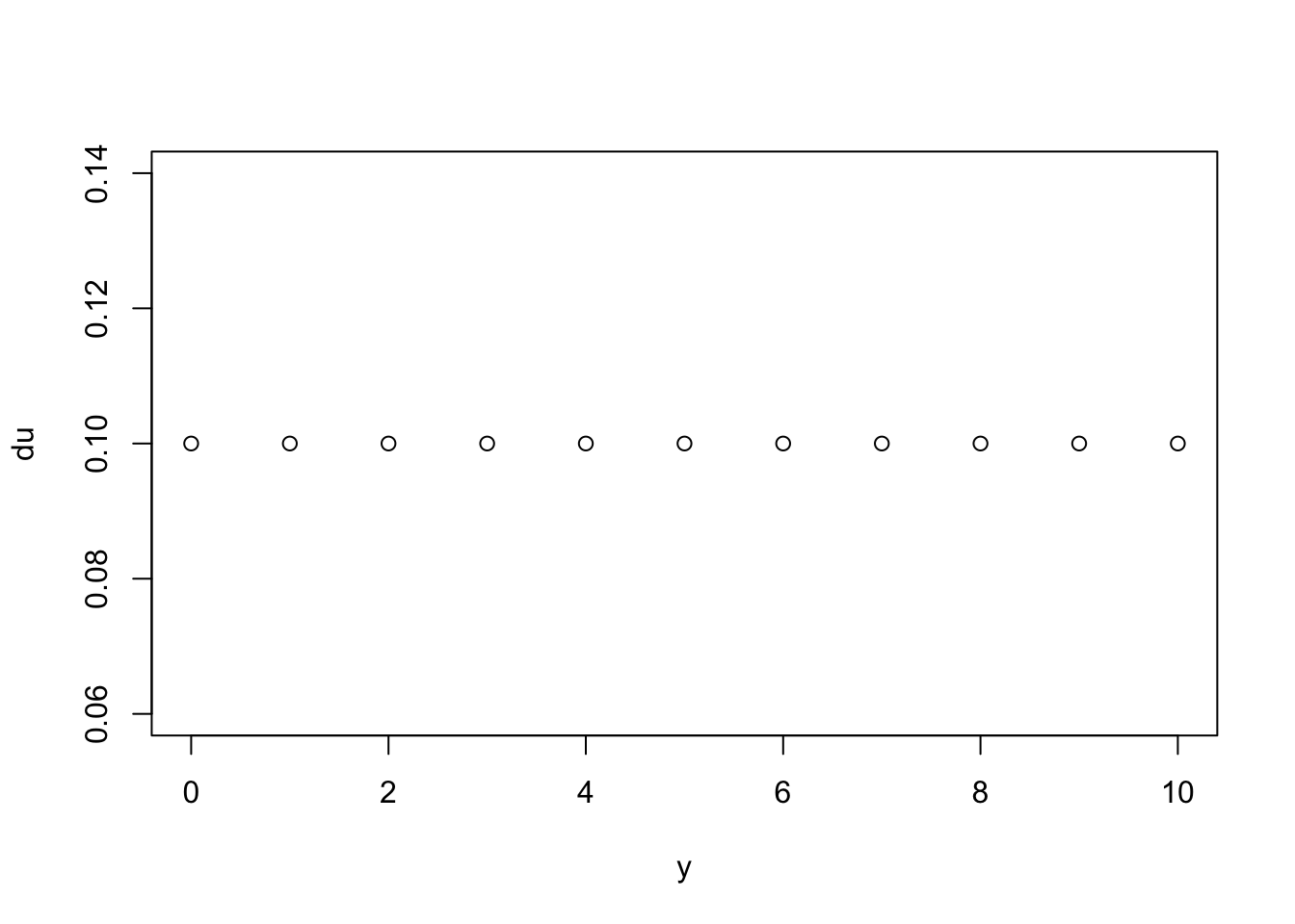
# normal distribution N(5,1) for sequence y
dn <- dnorm(y, mean = 5, sd = 1)
plot(y, dn)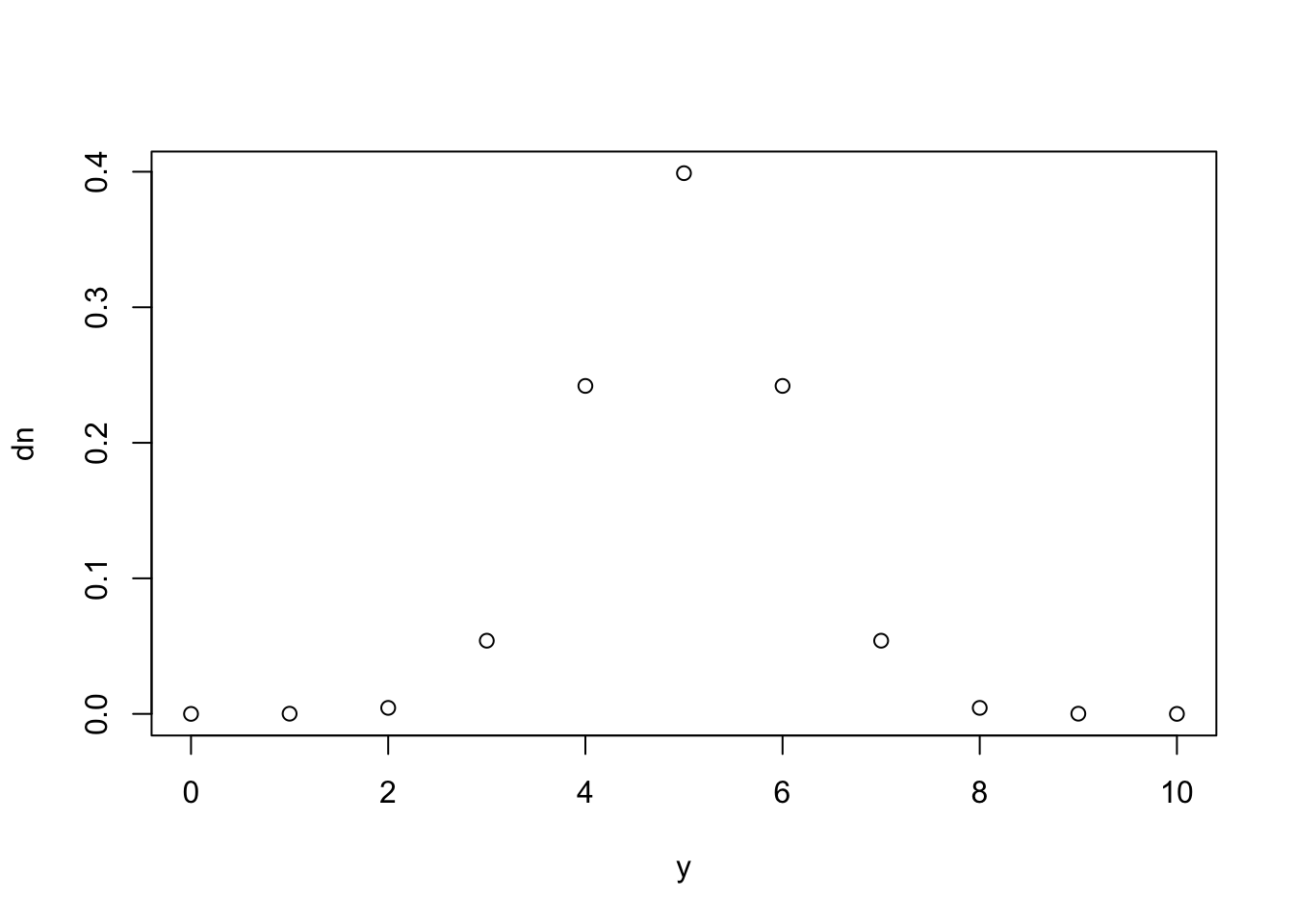
Other distributions can be accessed the same way: https://stat.ethz.ch/R-manual/R-devel/library/stats/html/Distributions.html.
Sampling from an array with a certain probability of obtaining each element:
# here sampling 1000 times
s <- sample(y, size = 1000, replace = TRUE, prob = dn)
hist(s)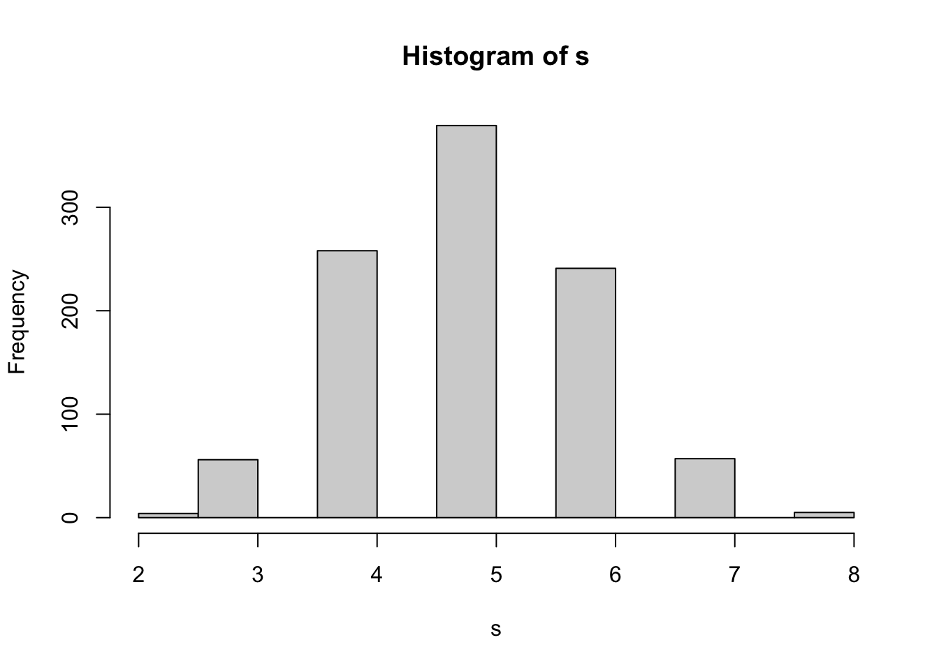
Copyright © 2024 Humboldt-Universität zu Berlin. Department of Geography.
![]()