- Packages
- Introduction
- Data
- Train-test splitting
- Tune SVM
- Model accuracy
- References
Machine Learning
Humboldt-Universität zu Berlin | Geography Department
Packages
library(e1071) # Support Vector Machines
library(caret) # confusion matrix
library(dplyr) # data wranling
Introduction
The primary goal of machine learning is to build models that make good predictions. This is not to say that statistical models that we used so far are not adequate for predictions, but their primary objective is statistical inference, i.e., understanding models and relationships. Balancing both goals is not easy. Thus, machine learning sacrifices inferences to predictive power. There are ways to interpret machine learning models, but inference is more challenging as we stray away from probabilistic frameworks.
Machine learning may use parametric models (e.g., logistic regression) and non-parametric models (e.g, random forest, support vector machine), or unsupervised models (k-means clustering). Hence, machine learning involves a wide range range of statistical (and computer science) tools that may require different strategies and workflows.
Support Vector Machine classification and regression is implemented
in a variety of packages. Here, we use the e1071 package,
which uses the libsvm library.
Data
For this exercise, we use the taxon data from the R Book
(Crawley, 2012).
taxa <- read.table("data/taxonomy.txt", header=T, stringsAsFactors = T)
head(taxa)
## Taxon Petals Internode Sepal Bract Petiole Leaf Fruit
## 1 I 5.621498 29.48060 2.462107 18.20341 11.27910 1.128033 7.876151
## 2 I 4.994617 28.36025 2.429321 17.65205 11.04084 1.197617 7.025416
## 3 I 4.767505 27.25432 2.570497 19.40838 10.49072 1.003808 7.817479
## 4 I 6.299446 25.92424 2.066051 18.37915 11.80182 1.614052 7.672492
## 5 I 6.489375 25.21131 2.901583 17.31305 10.12159 1.813333 7.758443
## 6 I 5.785868 25.52433 2.655643 17.07216 10.55816 1.955524 7.880880The dataset contains seven morphological variables
(Petals, Internode, Sepal,
Bract, Petiole, Leaf,
Fruit) that might be useful for separating the categorical
response variable Taxon. The Taxon variable is
a factor variable with four factor levels: I,
II, III, IV. The
table() function reveals that there are 30
individuals/observations per factor level.
table(taxa$Taxon)##
## I II III IV
## 30 30 30 30Train-test splitting
SVM requires tuning of hyperparameters. To avoid overfitting, we tune the model on a train dataset and validated it on a test dataset. Since, we only have a single dataset, we must split it into train and test data first.
The sample() function draws a random sample of
n units from a vector x, where x
is here a sequence vector ranging from 1 to N.
N <- 10
n <- 6
i <- sample(1:N, n)
i
## [1] 3 1 10 9 4 2We use a sequence vector, because we will not directly sample from
the dataset. Rather, we will create a random index vector i
that we can use to select training and the test data. Below is an
example, where x is the data vector we want to split
i indices the training samples and -iindices
the complement, i.e., the test samples.
x <- c(88, 11, 50, 113, 26, 20, 148, 142, 5, 32)
x[i]  # training data
## [1] 50 88 32 5 113 11x[-i] # test data## [1] 26 20 148 142Let’s apply this concept to our taxa data. We draw 60% of the samples for training, and we use the remaining 40% for testing.
train_id <- sample(nrow(taxa), round(0.5*nrow(taxa)))
df_train <- taxa[train_id,]
df_test <- taxa[-train_id,]
We can use the table function to see how the samples are distributed across our classes (taxa). Since we started out with a balanced sample (equal sample size per class), the training and test samples also should be roughly balanced.
table(df_train$Taxon)##
## I II III IV
## 13 16 17 14Finally, we must normalize the X
variables with a z-transformation. Recall, the SVM is a distance-based
classfier, which maximizes the distances from the support vectors to the
hyperplane. If we have variables with varying units and data ranges
(e.g., elevation and temperature), the classifier will only utilize the
variables with high value ranges. We can use the scale
function to do the normalization. We do not scale y, but we need to make sure that y is a factor variable when doing a
classification. Finally, we create variables X and y for training and testing. This step is
not needed, but it can be an easy and helpful way to document your
code.
X_train <- scale(dplyr::select(df_train, -Taxon))
X_test <- scale(dplyr::select(df_test, -Taxon))

y_train <- df_train$Taxon
y_test  <- df_test$Taxon
Tune SVM
The choice of the hyperparameters can significantly impact the accuracy of the model. To find the best hyperparameters, we can try-out different combinations of γ and C. This is called a grid-search. It is simple and effective, but it can be prohibitively computationally intensive with large numbers of parameters. Let’s define define different values for γ and C.
costs <- c(1, 5, 10, 15, 30, 60)
gammas <- c(0.1, 0.5, 0.14)
.. and do the gridsearch using the tune() function. We
also need to set the tunecontrol argument to specify the
k-fold cross validation used for assess model performance during the
tuning.
svm_tune <- tune(svm,
                 train.x=X_train,
                 train.y=y_train,
                 type = "C-classification",
                 kernel = "radial",
                 ranges = list(gamma = gammas, cost = costs),
                 tunecontrol = tune.control(cross = 5))
We can print the result of the tuning. The tuning step compares all models based on their overall accuracy using cross-validation. Here, the best model had a γ of 0.1 and a cost of 1. Also, the best performing model had an error rate of 0.1 or 10%.
svm_tune##
## Parameter tuning of 'svm':
##
## - sampling method: 5-fold cross validation
##
## - best parameters:
## gamma cost
## 0.1 1
##
## - best performance: 0.1Sometimes the lowest or highest parameters are picked. Here, the grid-search picked the lowest γ and C from our list. In this case, it is a good idea to expand the list to lower parameter values and re-run the grid-search.
costs <- c(0.01, 0.5, 1, 5, 10)
gammas <- c(0.01, 0.05, 0.1, 0.14)
svm_tune <- tune(svm,
                 train.x=X_train,
                 train.y=y_train,
                 type = "C-classification",
                 kernel = "radial",
                 ranges = list(gamma = gammas, cost = costs),
                 tunecontrol = tune.control(cross = 5))
svm_tune
##
## Parameter tuning of 'svm':
##
## - sampling method: 5-fold cross validation
##
## - best parameters:
## gamma cost
## 0.1 0.5
##
## - best performance: 0.06666667The second tuning results in lower error rates, and the selected
parameters are not onthe edges of the grid anymore. The tuning results
can nicely be visualized with the plot() function. The
graph below shows the error rate (1 - overall accuracy) of the
grid-search.
plot(svm_tune)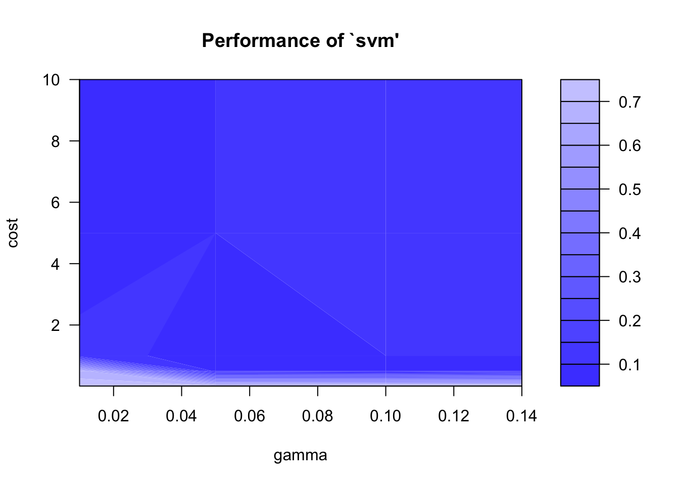
We can extract the best model from the tuning results as well:
svm_best <- svm_tune$best.model
summary(svm_best)
##
## Call:
## best.tune(METHOD = svm, train.x = X_train, train.y = y_train, ranges = list(gamma = gammas,
## cost = costs), tunecontrol = tune.control(cross = 5), type = "C-classification",
## kernel = "radial")
##
##
## Parameters:
## SVM-Type: C-classification
## SVM-Kernel: radial
## cost: 0.5
##
## Number of Support Vectors: 55
##
## ( 16 15 12 12 )
##
##
## Number of Classes: 4
##
## Levels:
## I II III IVModel accuracy
.. and estimate the model accuracy with the test dataset. The overall accuracy of the model is 0.95.
pred_best <- predict(svm_best, X_test)
confusionMatrix(data = pred_best, reference = y_test)
## Confusion Matrix and Statistics
##
## Reference
## Prediction I II III IV
## I 14 0 0 0
## II 0 14 0 0
## III 3 0 13 0
## IV 0 0 0 16
##
## Overall Statistics
##
## Accuracy : 0.95
## 95% CI : (0.8608, 0.9896)
## No Information Rate : 0.2833
## P-Value [Acc > NIR] : < 2.2e-16
##
## Kappa : 0.9334
##
## Mcnemar's Test P-Value : NA
##
## Statistics by Class:
##
## Class: I Class: II Class: III Class: IV
## Sensitivity 0.8235 1.0000 1.0000 1.0000
## Specificity 1.0000 1.0000 0.9362 1.0000
## Pos Pred Value 1.0000 1.0000 0.8125 1.0000
## Neg Pred Value 0.9348 1.0000 1.0000 1.0000
## Prevalence 0.2833 0.2333 0.2167 0.2667
## Detection Rate 0.2333 0.2333 0.2167 0.2667
## Detection Prevalence 0.2333 0.2333 0.2667 0.2667
## Balanced Accuracy 0.9118 1.0000 0.9681 1.0000References
Crawley, MJ (2012). The R Book. 2nd edition. John Wiley & Sons.
Copyright © 2024 Humboldt-Universität zu Berlin. Department of Geography.
![]()