Overview

Inverse Distance Weighted interpolation
Semivariogram
Kriging

Packages

We will mostly deal with package gstat, because it offers the widest functionality in the geostatistics curriculum for R: it covers variogram cloud diagnostics, variogram modeling, everything from global simple kriging to local universal cokriging, multivariate geostatistics, block kriging, indicator and Gaussian conditional simulation, and many combinations.

The functions in gstat take spatial vector and raster data as input. For spatial vector data, we already introduced the sf package (see this lab). In terms of raster data, gstat only understands formats from the older sp package and the newer stars package. All are from the same developers. The stars package was build to read and manipulate spatio-temporal array data (Pebesma, 2020). So this includes the usual raster data like satellite images and climate grids, but compared to other raster data packages, it extents the interface to incorporate the temporal dimension. Specifically, stars objects can have a time dimension in addition to the spatial 2D dimensions (longitude and latitude), where the time dimension can take Date values.

library("gstat")   # geostatistics
library("mapview") # map plot
library("sf")      # spatial vector data
library("stars")   # spatial-temporal data
library("terra")   # raster data handling 
library("ggplot2") # plotting
mapviewOptions(fgb = FALSE)

Data

For this tutorial, we use a dataset from Pebesma (2022). The dataset meuse is a tabular dataset (geopackage) that includes measurements of four heavy metals sampled from the top soil in a flood plain along the river Meuse. The dataset also contains a number of covariates. We also have a raster of some of the covariates meuse_gridcv. Further, we learn how to create our own grid for the sampled area: meuse_grid.

Meuse points

Let’s read the geopackage of the soil samples using the read_sf() function of the sf package (see this lab).

meuse <- read_sf('data/meuse.gpkg')
head(meuse)

## Simple feature collection with 6 features and 12 fields
## Geometry type: POINT
## Dimension:     XY
## Bounding box:  xmin: 181025 ymin: 333260 xmax: 181390 ymax: 333611
## Projected CRS: Double_Stereographic
## # A tibble: 6 × 13
##   cadmium copper  lead  zinc  elev    dist    om ffreq soil  lime  landuse dist_m
##     <dbl>  <dbl> <dbl> <dbl> <dbl>   <dbl> <dbl> <chr> <chr> <chr> <chr>    <dbl>
## 1    11.7     85   299  1022  7.91 0.00136  13.6 1     1     1     Ah          50
## 2     8.6     81   277  1141  6.98 0.0122   14   1     1     1     Ah          30
## 3     6.5     68   199   640  7.8  0.103    13   1     1     1     Ah         150
## 4     2.6     81   116   257  7.66 0.190     8   1     2     0     Ga         270
## 5     2.8     48   117   269  7.48 0.277     8.7 1     2     0     Ah         380
## 6     3       61   137   281  7.79 0.364     7.8 1     2     0     Ga         470
## # ℹ 1 more variable: geom <POINT [m]>

Spatial exploratory data analysis starts with the plotting of maps with a measured variable. Zinc concentration seems to be larger close to the river Meuse banks and in areas with low elevation.

mapview(meuse['zinc'])

Meuse grid

The meuse grid is a geotiff raster that contains five bands: 1) dist (distance to the Meuse river), 2) ffreq (flooding frequency class), 3) soil type, 4) part.a, and 5) part.b. The later two are arbitrary divisions of the area in two areas. We can read the grid using the read_stars() function.

meuse_gridcv <- read_stars("data/meuse_grid.tif")
meuse_gridcv

## stars object with 3 dimensions and 1 attribute
## attribute(s):
##                 Min.   1st Qu. Median      Mean 3rd Qu. Max.  NA's
## meuse_grid.tif     0 0.1192915      1 0.9884603       1    3 25045
## dimension(s):
##      from  to offset delta               refsys point           values x/y
## x       1  78 178440    40 Double_Stereographic FALSE             NULL [x]
## y       1 104 333760   -40 Double_Stereographic FALSE             NULL [y]
## band    1   5     NA    NA                   NA    NA part.a,...,ffreq

The resulting stars object now contains three dimension, where the bands are stored in the third dimension (here names band). To be able to use this grid in gstat, we need to split the bands into separate attributes:

meuse_gridcv <- split(meuse_gridcv, "band")
meuse_gridcv

## stars object with 2 dimensions and 5 attributes
## attribute(s):
##         Min.   1st Qu.   Median      Mean  3rd Qu.     Max. NA's
## part.a     0 0.0000000 0.000000 0.3986465 1.000000 1.000000 5009
## part.b     0 0.0000000 1.000000 0.6013535 1.000000 1.000000 5009
## dist       0 0.1192915 0.271535 0.2971195 0.440159 0.992607 5009
## soil       1 1.0000000 1.000000 1.5775056 2.000000 3.000000 5009
## ffreq      1 1.0000000 2.000000 2.0676764 3.000000 3.000000 5009
## dimension(s):
##   from  to offset delta               refsys point x/y
## x    1  78 178440    40 Double_Stereographic FALSE [x]
## y    1 104 333760   -40 Double_Stereographic FALSE [y]

Create a grid

Spatial interpolation is done on a regular grid. The routines in gstat require you to specify such a grid as a stars object (or the older sp object). If you have an existing raster dataset, you can use that as a template. Perhaps that raster dataset also contains covariates that you want to include in the modeling like meuse_gridcv. Alternatively, you can create your own grids with varying spacings between cells and a specified extent.

There are different ways to create a regular grid in R. The sf package also includes useful functions like st_make_grid(). Here, we use a simpler way that does not require sf. Let’s start by grabing the bounding box coordinates of the soil samples (meuse) to define the extent of the output grid.

bbox <- st_bbox(meuse)
bbox

##   xmin   ymin   xmax   ymax 
## 178605 329714 181390 333611

We can access the elements of bbox by name, e.g. bbox$xmin. With the seq() function, we can then create a sequence of regularly spaced coordinates in the x and y direction. Here, I use an increment of 40, which defines the cell size.

cell_size <- 40

x <- seq(bbox$xmin, bbox$xmax, by=cell_size)
y <- seq(bbox$ymin, bbox$ymax, by=cell_size)

With expand.grid(), we can combine every x coordinate with every y coordinate. This yields a regular grid of coordinates. The output of the function is a data.frame with the expanded columns x and y columns.

meuse_grid <- expand.grid(x=x, y=y)
plot(meuse_grid$x, meuse_grid$y, pch=19, cex=0.1)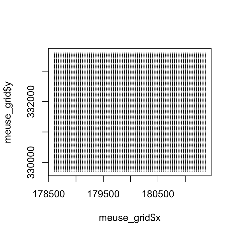

Now, we can convert the data.frame containing the grid coordinates to a stars object using st_as_stars(). But first, I add a column tmp with some fake value. Otherwise the stars object would have 0 attributes and that would fail the interpolation functions.

meuse_grid$tmp <- 1
meuse_grid <- st_as_stars(meuse_grid, crs=st_crs(meuse))
st_crs(meuse_grid) <- st_crs(meuse) # re-assign crs to be safe

IDW interpolation

Inverse distance-based weighted interpolation (IDW) computes a weighted average,

\[\begin{equation} \hat{Z}(s_0) = \frac{\sum_{i=1}^{n}w(s_i)Z(s_i)}{\sum_{i=1}^{n}w(s_i)} \end{equation}\]

where weights for observations are computed according to their distance to the interpolation location,

\[w(s_i) = ||s_i-s_0||^{-p}\]

with $|| ? ||$ indicating Euclidean distance and $p$ an inverse distance weighting power, defaulting to 2. If $s_0$ coincides with an observation location, the observed value is returned to avoid infinite weights. The inverse distance power determines the degree to which the nearer point(s) are preferred over more distant points; for large values IDW converges to the one-nearest-neighbor interpolation.

The corresponding gstat function is idw(). The function takes a formula, a location dataset (sf) and a grid (stars). The formula objects is consistent with the formulas we used for specifying regression models. So, here we predict zinc (response). The ~ 1 part means that we do not include any additional predictors/covariates. The predictions are only based on the spatial locations.

zn.idw <- gstat::idw(zinc ~ 1, locations=meuse, newdata=meuse_gridcv, idp = 2)

## [inverse distance weighted interpolation]

The output is a stars object with two attributes: 1) var1.pred contains the predicted values, and 2) var1.var contains the variance estimates. The statistics of var1.var are NA because inverse distance does not provide prediction error variances.

zn.idw

## stars object with 2 dimensions and 2 attributes
## attribute(s):
##                Min.  1st Qu.   Median     Mean  3rd Qu.     Max. NA's
## var1.pred  128.4345 293.2323 371.4119 423.1647 499.8198 1805.776 5009
## var1.var         NA       NA       NA      NaN       NA       NA 8112
## dimension(s):
##   from  to offset delta               refsys x/y
## x    1  78 178440    40 Double_Stereographic [x]
## y    1 104 333760   -40 Double_Stereographic [y]

We can plot the predictions. Here, I first convert them with rast() to a SpatRaster from the terra package. Overplotting the sample locations didn’t work right otherwise. This is a bug and should probably not be needed, but the example shows that you can convert back and forth between stars and terra.

plot(rast(zn.idw["var1.pred"]))
plot(meuse["zinc"], col=1, cex=0.5, add=T, type="p")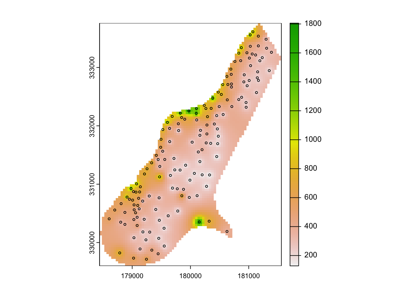

# mapview(zn.idw, zcol='var1.pred', layer.name = "Zinc ppm")

IDW considers only distances to the prediction location and thus ignores the spatial configuration of observations. This may lead to undesired effects if the observation locations are strongly clustered.

Notably, IDW weights are guaranteed to be between 0 and 1, resulting in interpolated values never outside the range of observed values.

Stationarity

The spatial correlation between two observations of a variable $z(s)$ at locations $s_1$ and $s_2$ cannot be estimated, as only a single pair is available. To obtain the necessary replication, we need to replicate the experiment with multiple samples from multiple locations. But to do that, we need to assume that the spatial process is the same at all those locations. In other words, we need to make stationarity assumptions about our spatial process.

Stationarity means that characteristics of a random function (our spatial process that generates a variable) stay the same when shifting a given set of $n$ points from one part of a region to another. The spatial process is called strictly stationary if for any set of $n$ points $s_1,..., s_n$ the multivariate distribution does not change. In other words, everything looks the same everywhere and anytime. Well, this may not seem like a reasonable assumption for geographic processes.

A less restrictive condition is given by weak stationarity, which is also called second-order stationarity because it only assumes stationarity of the first two moments of the distribution. That is, the spatial process has a constant mean $E[Z(x)]$ and variance $Var[Z(x)]$. Also, the covariance between two observations separated by a distance $h$: $cov(Z(x+h), Z(x))$ only relies on the distance $h$ between the observations and not on the spatial location $x$ inside the region.

A specific type of second-order stationarity, and most important for the variogram analysis, is called intrinsic stationarity. Here, we assume second-order stationarity of the differences between pairs of values at two locations: $Z(x+h)−Z(x)$. We are not interested in $Z(x)$ but in the differences. Again, this implies the assumption that the variance of these differences does not depend on location but only depends on separation distance $h$:

\[Var(Z(x+h)−Z(x))=2\gamma(h)\]

Lagged scatter plots

A simple way to acknowledge that spatial correlation is present or not is to make scatter plots of pairs $Z(s_i)$ and $Z(s_j)$, grouped according to their separation distance $h_{ij} = || {s_{i} - s_{j}} ||$.

gstat::hscat(log(zinc) ~ 1, meuse, (0:9) * 100)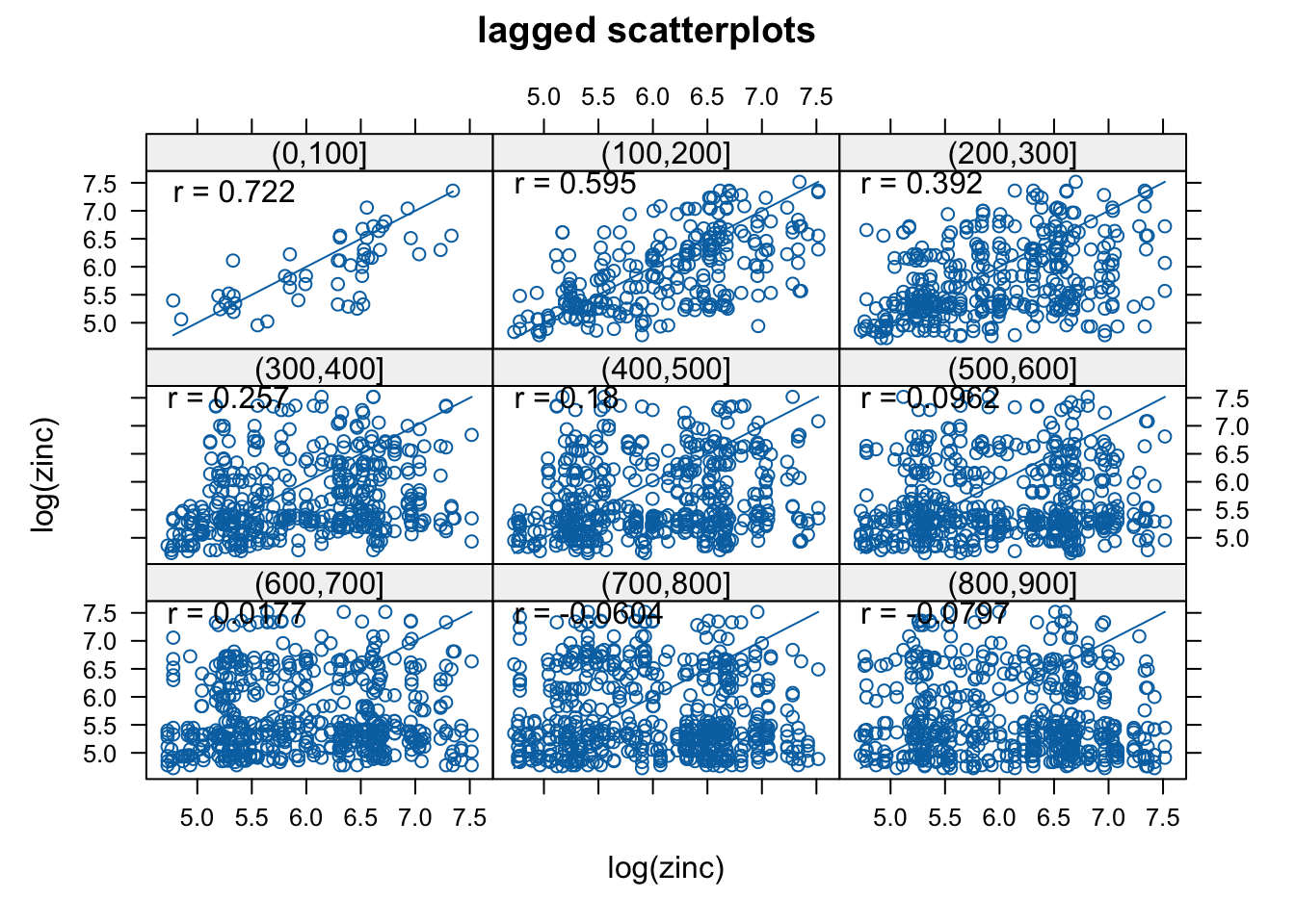

Variogram cloud

We can plot the difference between pairs of sample values as a function of separation distance $h$. The so-called variogram cloud plots all possible squared differences of observation pairs $(Z(x) - Z(x+h))^2$ against their separation distance $h$. The difference is divided by 2 to account for the fact that two points share this value. Hence, $\gamma$ is often called semi-variance (half the variance).

\[\gamma_h=\frac{1}{2}(Z(x) - Z(x+h))^2\]

meuse.vc <- variogram(log(zinc) ~ 1, meuse, cloud = TRUE)
plot(meuse.vc, ylab=bquote(gamma), xlab=c("h (separation distance in m)"))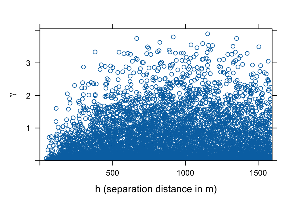

Since $\gamma$ is a difference it is a measure of dissimilarity, i.e., the smaller the dissimilarity the more similar are observations. Thus, the variogram cloud allows you to observe if sample pairs closer to each other are more similar than pairs further apart, which is usually the case. The variogram cloud also allows you to observe the distribution of dissimilarity at particular distances. For example, the variogram cloud above shows that $\gamma$ has a skewed distribution at any distance. That is, the majority of plots are similar even at higher distances. However, dissimilarity increases with distances up to 500 m or so.

Sample variogram

In geostatistics the spatial correlation is often modeled from the sample variogram. The sample variogram plots averages of the variogram cloud values over distance intervals $h$. If we further assume isotropy, which is direction independence of semivariance, we can replace the vector $h$ with its length, $||h||$.

Under this assumption, the variogram can be estimated from $N_h$ sample data pairs $z(x)$, $z(x + h)$ for a number of distances (or distance intervals) $\tilde{h}_j$ by:

\[\hat{\gamma}(\tilde{h}_j) = \frac{1}{2N_h}\sum_{i=1}^{N_h}(Z(x)-Z(x+h))^2\]

You can construct a sample variogram() in R using the variogram function of the gstat package. The ~ 1 defines a single constant predictor leading to a spatially constant mean coefficient.

meuse.v <- gstat::variogram(log(zinc) ~ 1, meuse)
plot(meuse.v, ylab=bquote(gamma), xlab=c("h (separation distance in m)"))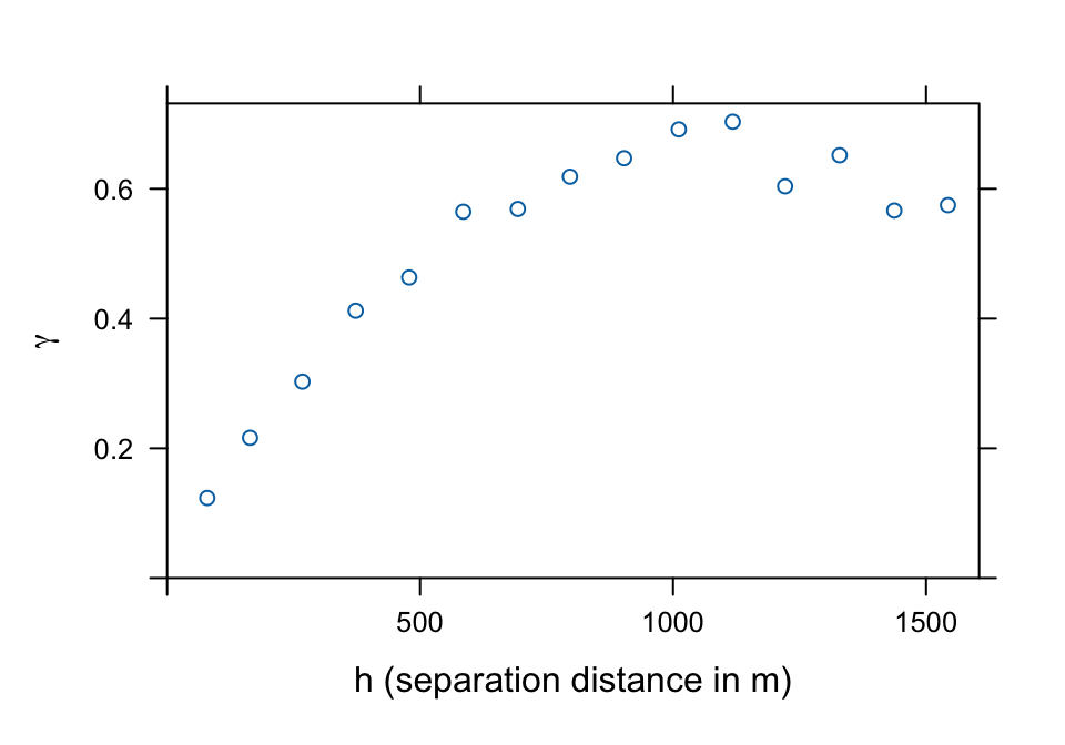

Direction dependence

The previously used variogram function makes a number of decisions by default. It decides that direction is ignored: point pairs are merged on the basis of distance, not direction. An alternative is, for example to look in four different angles by specifying the alpha keyword.

plot(variogram(log(zinc) ~ 1, meuse, alpha = c(0, 45, + 90, 135)))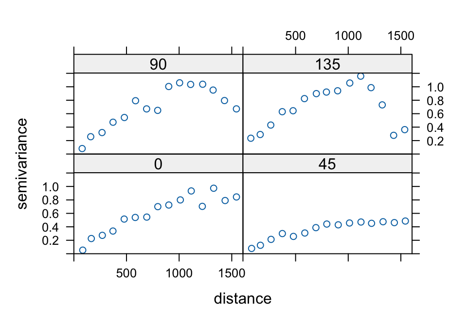

Cutoff and lag width

A similar issue is the cutoff distance, which is the maximum distance up to which point pairs are considered and the width of distance interval over which point pairs are averaged in bins. The default value gstat uses for the cutoff value is one third of the largest diagonal of the bounding box (or cube) of the data. Good reasons to decrease the cutoff may be when a local prediction method is foreseen, and only semivariances up to a rather small distance are required. For the interval width, gstat uses a default of the cutoff value divided by 15.

plot(variogram(log(zinc) ~ 1, meuse, cutoff = 1000, width = 50))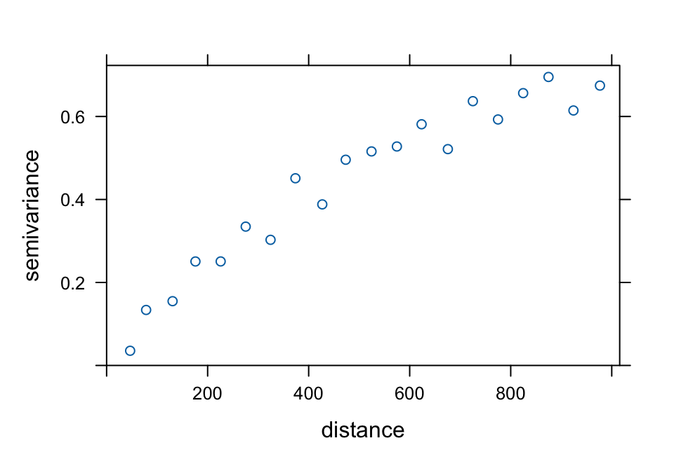

Theoretical variogram

Using the sample variogram (also called experimental variogram), we can fit a theoretical variogram model to estimate a number of parameters that describe the range of autocorrelation and variance:

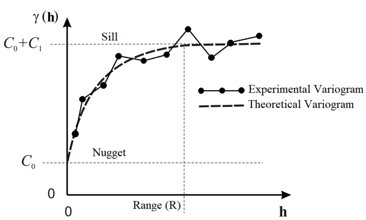
$R$ is the range of spatial auto-correlation, i.e., sample locations separated by distances closer than R are spatially auto-correlated, whereas locations farther apart than R are not.
$C_0$ is the nugget effect, which can be attributed to measurement errors or spatial sources of variation at distances smaller than the sampling interval.
$C_1$ is the partial sill (sill minus nugget).
$C_0+C_1$ is the sill, which is the modeled semi-variance at range $R$.

A wide range of variogram models are available for estimating these parameters, e.g., linear, spherical, exponential, Gaussian. Note, the exponential, Gaussian, and Bessel model reach their sill asymptotically (as $h \to \infty$). For an overview of all available variogram models in R, type in the command line vgm() without any model arguments.

Pebesma, E. (2014): gstat user’s manual

Use the vgm() function to construct a variogram model by specifying the nugget $C_0$, partial sill $C_1$ (psill), range $R$, and the model form.

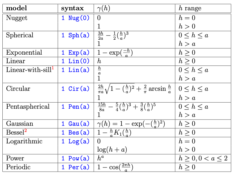
myVariogramModel <- vgm(psill=1, "Sph", range=100, nugget=0.5)

plot(myVariogramModel, cutoff=150)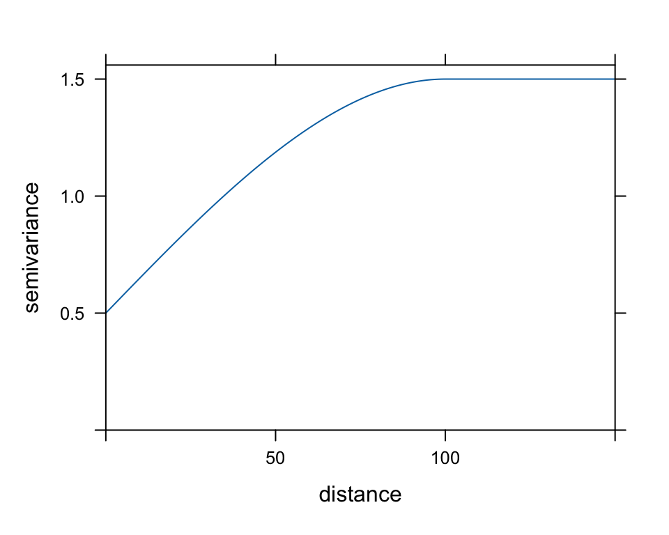

A visual overview of the basic variogram models available in gstat can be obtained as follows:

show.vgms()

Fit a variogram

For weighted least squares fitting of a variogram model to the sample variogram, we need to take several steps: 1) calculate the sample variogram, 2) choose a suitable model, 3) choose initial parameters for our model, 4) and fit the model.

Calculate the sample variogram

meuse.v <- variogram(log(zinc) ~ 1, meuse)

Choose a suitable model (e.g. exponential, spherical), with or without nugget
Choose suitable initial values for partial sill(s), range(s), and possibly nugget

Let’s try the the spherical model with and some initial guesses for the parameters. Looking at the sample variogram, good initial values for the nugget may be 0.1, for the partial sill (sill minus nugget) = 0.6, and for the range perhaps 800m. We can plot both, the sample variogram and model on top of each other to evaluate our initial model.

meuse.sph <- vgm(psill=0.6, "Sph", range=800, nugget=0.1)
plot(meuse.v, meuse.sph, cutoff=1000)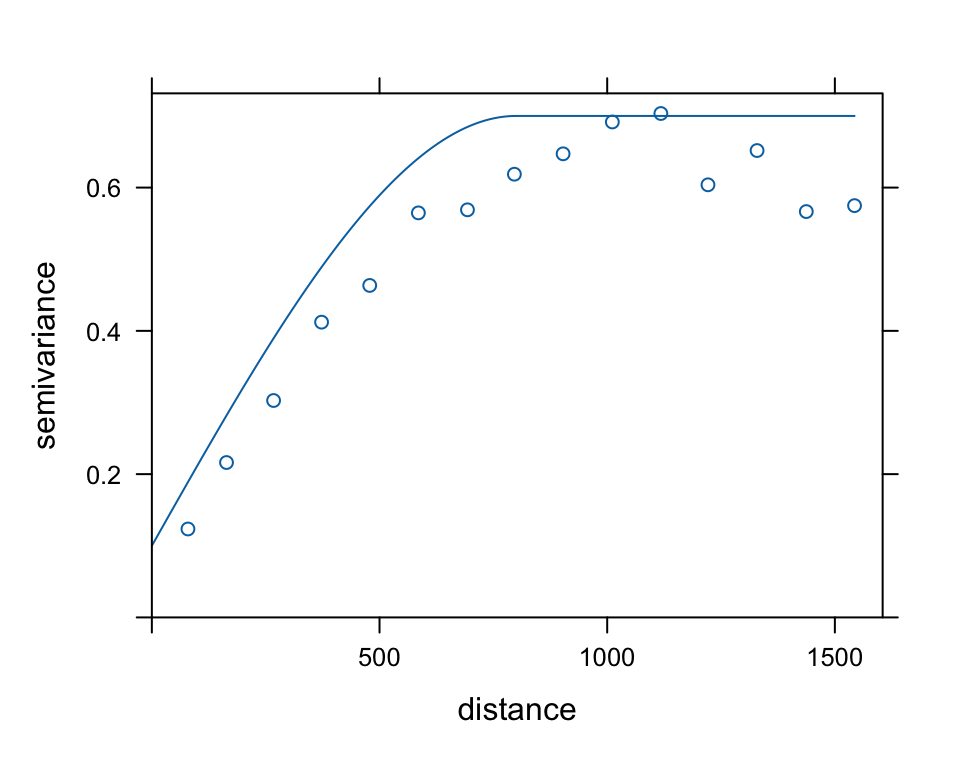

Fit this model using one of the fitting criteria

meuse.vfit <- fit.variogram(meuse.v, meuse.sph)
meuse.vfit

##   model      psill    range
## 1   Nug 0.05065661   0.0000
## 2   Sph 0.59060200 896.9784

Let’s plot the fitted variogram over the sample variogram:

plot(meuse.v, meuse.vfit)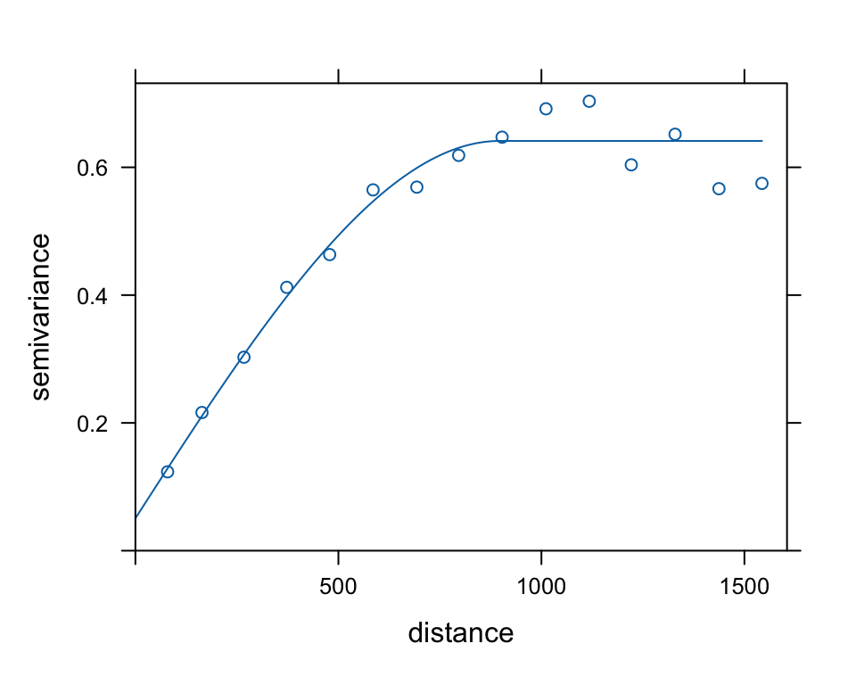

Model fitting may fail if we choose initial values too far off from reasonable values.

fit.variogram(meuse.v, vgm(1, "Sph", 10, 1))

## Warning in fit.variogram(meuse.v, vgm(1, "Sph", 10, 1)): singular model in variogram fit

##   model psill range
## 1   Nug     1     0
## 2   Sph     1    10

Partial variogram model fitting

Also partial fitting of variogram coefficients can be done with gstat. Suppose we know for some reason that the partial sill for the nugget model (i.e. the nugget variance) is 0.06, and we want to fit the remaining parameters. Alternatively, the range parameter(s) can be fixed using argument fit.ranges.

fit.variogram(meuse.v, vgm(0.6, "Sph", 800, 0.06), fit.sills = c(FALSE, TRUE))

##   model     psill    range
## 1   Nug 0.0600000   0.0000
## 2   Sph 0.5845857 923.0126

Visual variogram model fitting

An alternative approach to fitting variograms is by visual fitting, the so-called eyeball fit. Package geoR provides a graphical user interface for inter-actively adjusting the parameters:

library(geoR)
library(sp)

meuse_sp <- as(meuse["zinc"], "Spatial")
v.eye <- eyefit(variog(as.geodata(meuse_sp), max.dist = 1500))
ve.fit <- as.vgm.variomodel(v.eye[[1]])

Typically, visual fitting will minimize $|\gamma(h) - \hat{\gamma}(h)|$ with emphasis on short distance/small $\gamma(h)$ values, as opposed to a weighted squared difference, used by most numerical fitting. An argument to prefer visual fitting over numerical fitting may be that the person who fits has knowledge that goes beyond the information in the data.

Ordinary kriging

Kriging utilizes the theoretical variogram to interpolate values at any location based on distant-variance relationship. We’ll perform Ordinary Kriging at the meuse grid locations. Recall, ordinary kriging has a constant intercept, denoted in the formula with ~ 1:

# create sample variogram
meuse.v <- gstat::variogram(log(zinc) ~ 1, meuse)

# fit variogram model
meuse.vfit <- gstat::fit.variogram(meuse.v, vgm(1, "Sph", 800, 1))

# ordinary kriging
lz.ok <- gstat::krige(log(zinc) ~ 1, meuse, meuse_gridcv, meuse.vfit)

## [using ordinary kriging]

plot(rast(lz.ok['var1.pred']))
plot(meuse["zinc"], col="blue", cex=0.5, type="p", add=T)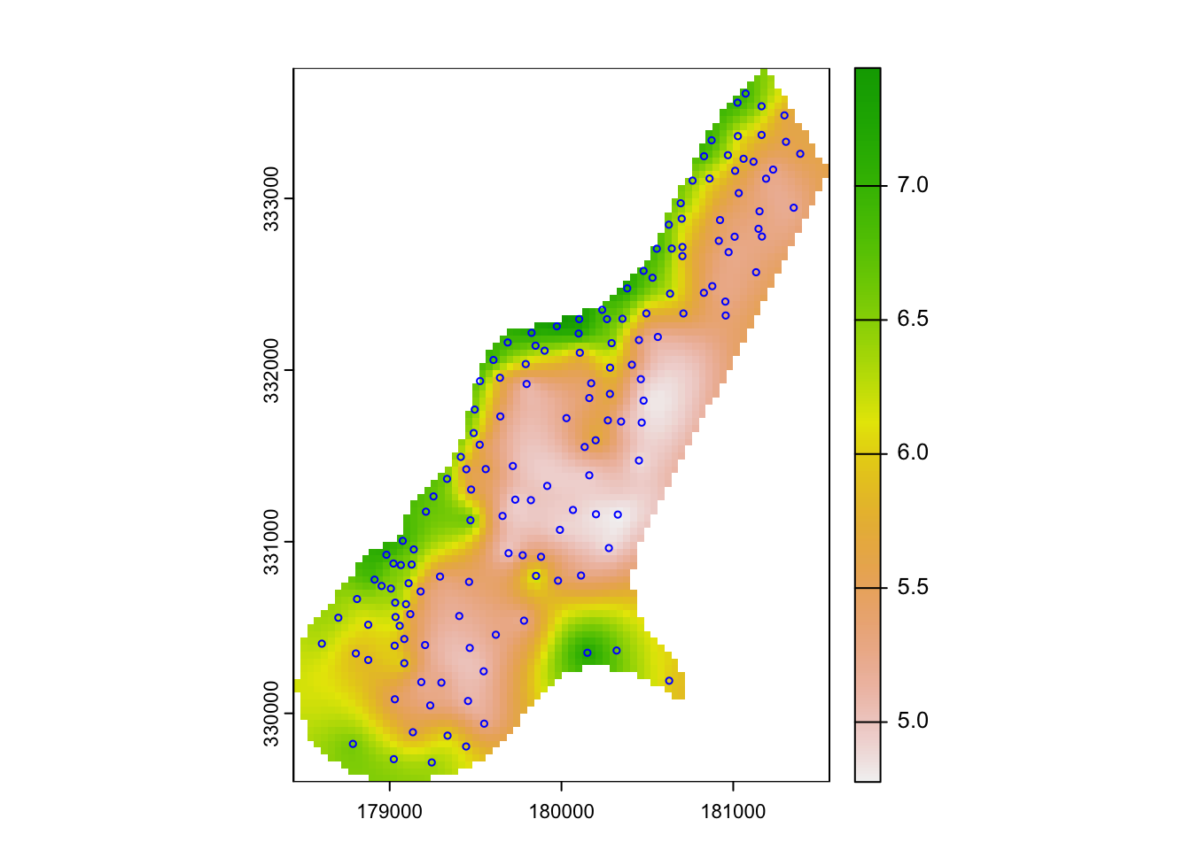

# mapview(lz.ok, zcol='var1.pred') # + mapview(meuse, zcol='zinc')

Kriged maps using a variogram with no or a small nugget are typically very similar to inverse distance interpolation results.

The lz.ok object stores not just the interpolated values, but the variance values as well. These can be passed to the raster object for mapping as follows:

plot(rast(lz.ok['var1.var']))
plot(meuse["zinc"], col="blue", cex=0.5, type="p", add=T)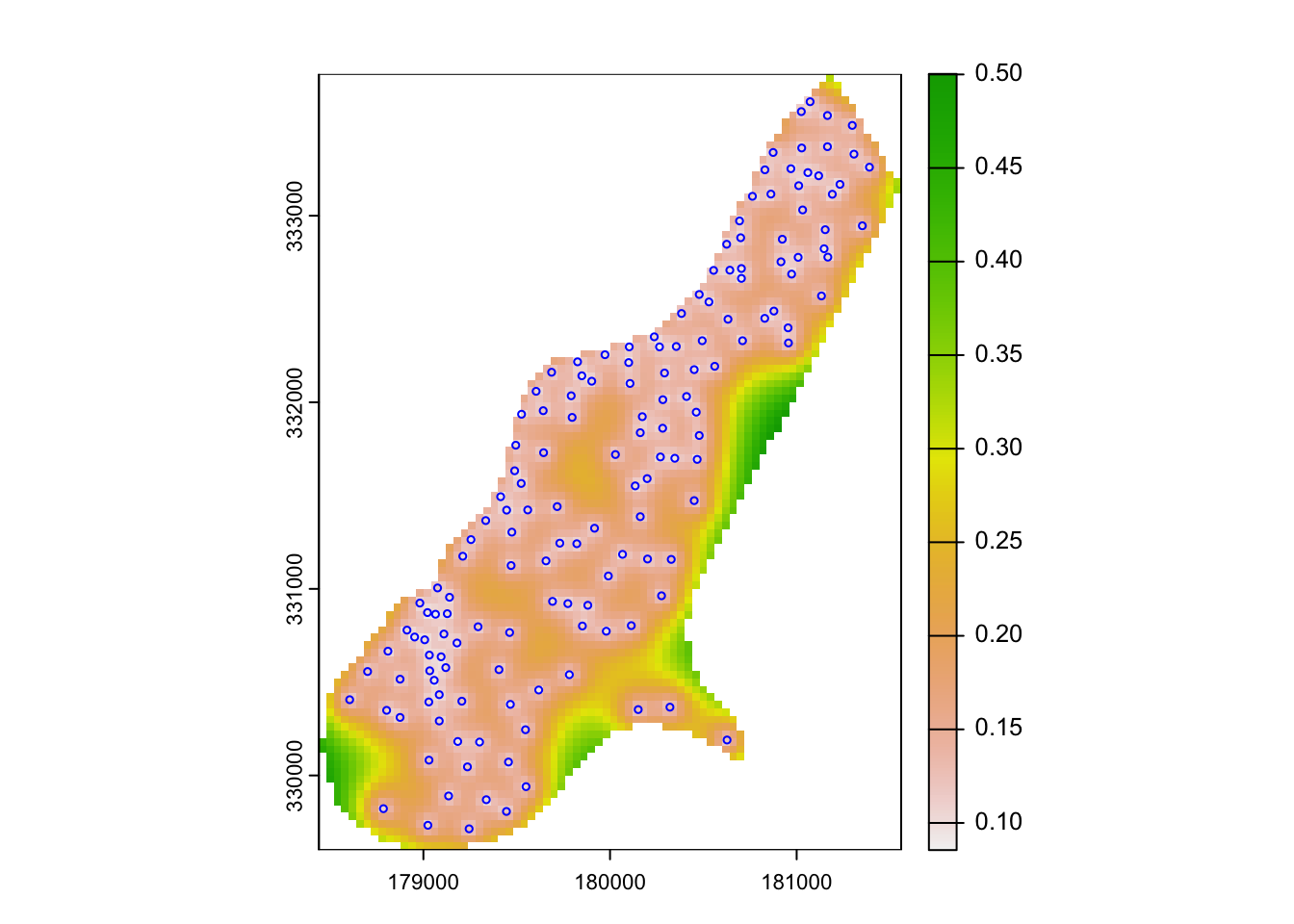

Universal kriging

Universal kriging includes other covariates to account for potential trends, e.g. here with distance to the river meuse.

# create sample variogram
meuse.rv <- variogram(log(zinc) ~ sqrt(dist), meuse)

# fit variogram model
meuse.rvfit <- fit.variogram(meuse.rv, vgm(1, "Sph", 300, 1))

To apply the model spatially, we also need a grid of those covariates. Recall meuse_gridcv is a raster of different covariates over the study area including a band/attribute of distance to the river (dist).

plot(meuse_gridcv["dist"])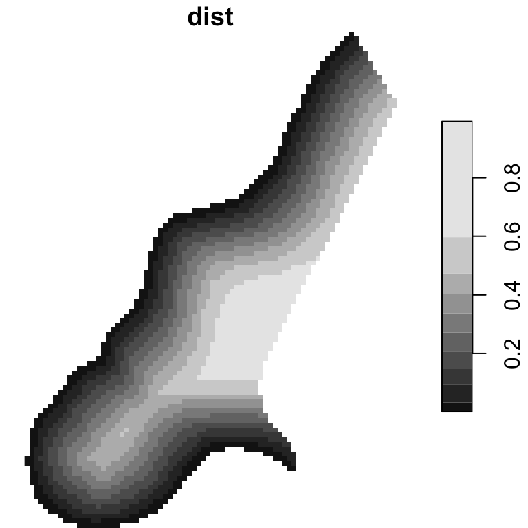

Let’s apply the model for universal kriging using the variogram model and the distance raster:

lz.uk <- krige(log(zinc) ~ sqrt(dist), locations=meuse, 
                                       newdata=meuse_gridcv, 
                                       model=meuse.rvfit)

## [using universal kriging]

..and plot the results.

plot(rast(lz.uk["var1.pred"]))
plot(meuse["zinc"], col="red", cex=0.5, type="p", add=T)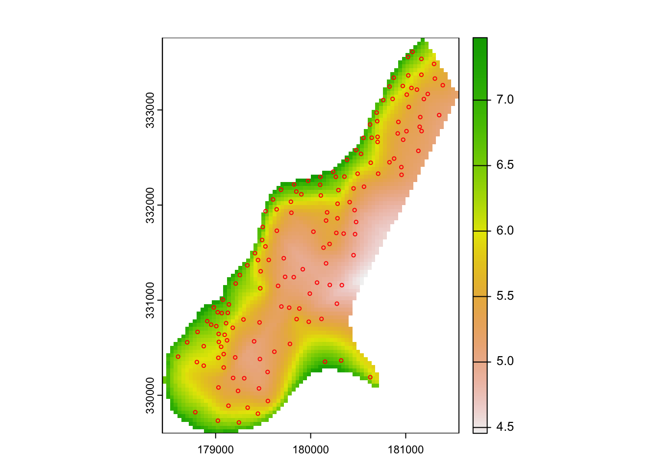

Comparison

Comparison of IDW and Kriging results. The graph shows from left to right, IDW, Ordinary Kriging and Universal Kriging results.

# simple back-transformation
lz.uk_pred <- exp(rast(lz.uk["var1.pred"]))
lz.ok_pred <- exp(rast(lz.ok["var1.pred"]))

# stack all three rasters
pred_stack <- c(rast(zn.idw["var1.pred"]), 
                lz.ok_pred, 
                lz.uk_pred)
names(pred_stack) <- c("IDW", "OK", "UK")

plot(pred_stack, nc=3, range = c(0, 2000), axes=F)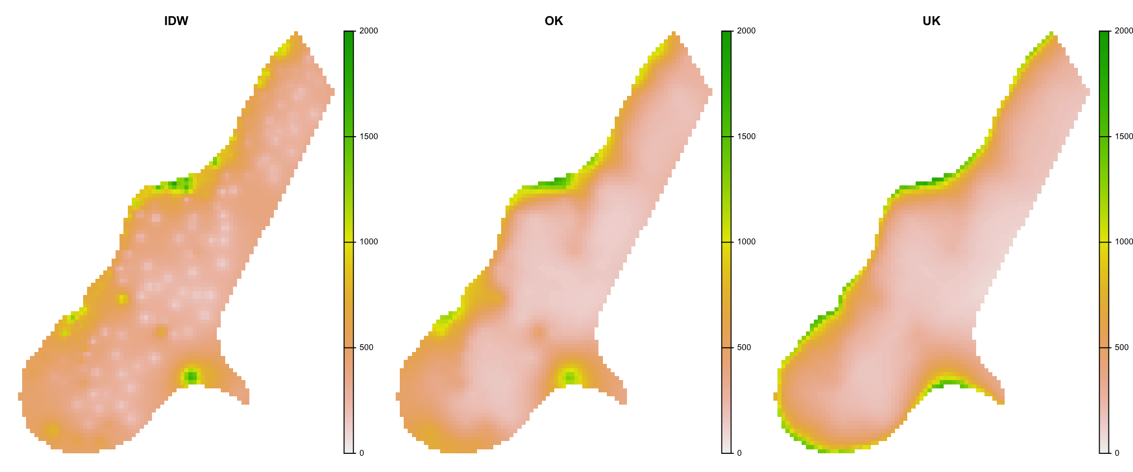

References

Bivand, R. S., Pebesma, E., Gómez-Rubio, V. (2013): Applied Spatial Data Analysis with R. Second Edition. Springer
Gimond, M. (2020): Intro to GIS and Spatial Analysis
Pebesma, E. (2014): gstat user’s manual.
Pebesma, E. (2018). Simple Features for r: Standardized Support for Spatial Vector Data. R Journal 10 (1).
Pebesma, E. (2022): The meuse data set: a brief tutorial for the gstat R package.
Pebesma, E. (2022): stars: Spatiotemporal Arrays, Raster and Vector Data Cubes.
Wackernagel, H. (2003): Multivariate Geostatistics: An Introduction with Applications. 3rd edition. Springer

Spatial interpolation in R

Humboldt-Universität zu Berlin | Geography Department