- Packages
- Raster data
- The
terrapackage
- SpatRaster from scratch
- Manipulate SpatRaster
- Read SpatRaster from a filename
- Plot a map
- rasterVis
- Write SpatRaster
- Sampling
- Predict
- Reading
Raster Data in R
Humboldt-Universität zu Berlin | Geography Department
Packages
library(terra)
library(rasterVis)
Raster data
Today, we’ll work with spatial data in R. One special type of spatial data are raster. Raster consist of cells (pixels) that are arranged as rows and columns in a regular grid. Examples of raster data are digital elevation models (DEM), gridded climate or meteorological variables, satellite images, discrete maps such as land cover maps, and continuous maps of vegetation cover, biophysical variables, and soil variables. Common raster file formats are the GeoTiff (suffix .tif), IMAGINE (suffix .img), and NetCDF (suffix .nc). There are many more formats, but most of them can be read and written in R.
The terra package
The terra package is the main package for creating,
reading, manipulating, and writing raster data. The terra
package supersedes the older raster package developed by
the same team of authors. Because raster has been around
for a longer time, dependencies with some packages may still exist. But
development of raster will eventually be stopped at some
point. You can install the latest version of terra from
CRAN with install.packages("terra"). You’ll find an online
documentation of the package here. I also recommend you scroll
through the package description to get a first overview of the
functationality of the package.
?`terra-package`The terra package defines a number of spatial classes.
The most important ones are:
SpatRasterto store raster dataSpatVectorto store spatial vector data, i.e., points, lines, polygons.SpatExtentto store information on spatial extent
SpatRaster from scratch
The rast function creates a SpatRaster object. One can
create a SpatRaster from scratch, from a filename, or from another
object. Below, we create a SpatRaster from scratch by specifying
dimensions and spatial extent.
r <- rast(nrows=40, ncols=20, xmin=0, xmax=10, ymin=0, ymax=10)
r
## class : SpatRaster
## dimensions : 40, 20, 1 (nrow, ncol, nlyr)
## resolution : 0.5, 0.25 (x, y)
## extent : 0, 10, 0, 10 (xmin, xmax, ymin, ymax)
## coord. ref. : lon/lat WGS 84 (CRS84) (OGC:CRS84)Object r has the structure of a SpatRaster but it does
not contain any values. We can access the values of a SpatRaster with
the function values. Here, we create a vector of random
numbers with a length that is equal to the number of raster cells and
assign it to the pixel values of the SpatRaster object.
values(r) <- runif(ncell(r))Similarly, we can extract the values of a SpatRaster and assign them
to a numerical vector v. You’ll see v is
actually a matrix with the dimensions (x, y), where x is the number of
cells in a layer, and y is the number of layers. The SpatRaster
r has 800 cells (pixels) and 1 layer.
v <- values(r)
dim(v)
## [1] 800 1head(v)## lyr.1
## [1,] 0.1698094
## [2,] 0.4494488
## [3,] 0.8624731
## [4,] 0.9194103
## [5,] 0.2338003
## [6,] 0.5710324We can plot the SpatRaster object using the familiar plot function.
plot(r)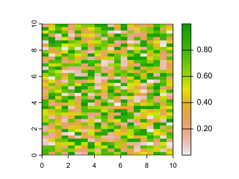
Manipulate SpatRaster
You can manipulate the pixel values of that layer by applying basic functions and operations.
q <- 100 * r^2
plot(q)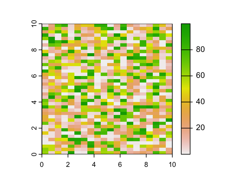
# create a binary mask based on a logical expression
m <- q < 10
plot(m)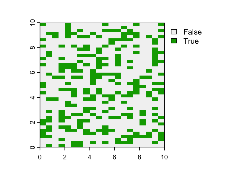
Our SpatRaster r and q have only a single
layer. We can stack both layers together using the concatenate function
c().
p <- c(r, q)

# assign meaningful names to the layers
names(p) <- c("random", "scaled_random")

plot(p)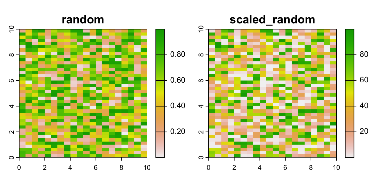
Summary functions (min, max,
mean, prod, sum,
median, cv, any,
all) yield a single value for every pixel (or two values
when using range). So, they always return a SpatRaster
object with a single layer (or two layers in case of
range). The following code calculates for every pixel in
SpatRaster p, the mean value across the two layers.
ma <- mean(p)
plot(ma)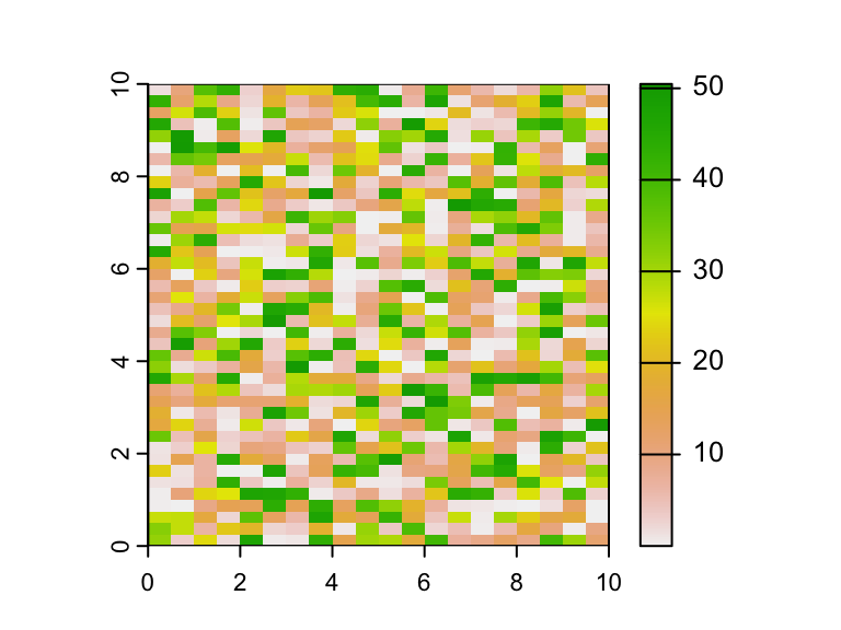
If you want a single value summarizing all pixel values, e.g. mean
pixel value for each layer, use global.
global(p, fun="mean")## mean
## random 0.5116364
## scaled_random 34.4984523You can also use the square brackets to access and replace values in a raster. The example below shows how to truncate a value range, i.e., all values less than 0.5 are replaced with the value 0.5.
r[r < 0.5] <- 0.5
plot(r, range=c(0,1))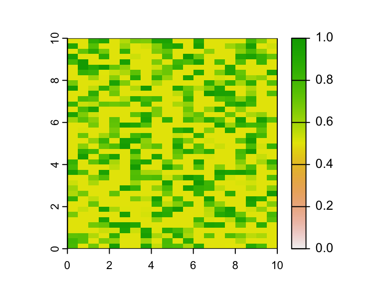
The function app provides a more generic interface to do
a computation for a single SpatRaster. The function takes a SpatRaster
and the function you want to apply. The function below replace all
values less than and equal to 0.5 with NA. Note, this is just a simple
example. The idea here is to facilitate the application of more complex
functions from you or other packages.
myFunction <- function(x){ x[x <= 0.5] <- NA; return(x)}
w <- app(r, fun= myFunction)
plot(w, range=c(0,1))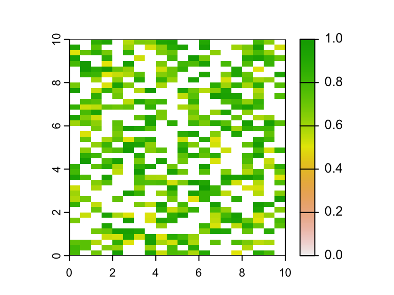
Read SpatRaster from a filename
Usually, we create a SpatRaster object from a filename. The resulting
object (here s) represents a connection to the physical
file on disc, but does not store the file in memory. This is helpful
when opening large raster files. Type the object into the console to
print important metadata of the raster including dimensions, coordinate
reference system, extent, layer names, etc.
s <- rast("Data/bioclim_subset.tif")
s
## class : SpatRaster
## dimensions : 150, 150, 4 (nrow, ncol, nlyr)
## resolution : 5000, 5000 (x, y)
## extent : 4896250, 5646250, 2405250, 3155250 (xmin, xmax, ymin, ymax)
## coord. ref. : ETRS89 / LAEA Europe
## source : bioclim_subset.tif
## names : Annual ~erature, Max Tem~t Month, Min Tem~t Month, Annual ~itation
## min values : 0.52425, 11.46267, -13.190, ?
## max values : 12.17329, 28.64300, -4.343, ?White space in layer names may cause problems down the line. It is a good idea to replace layer names with shorter but meaningful names.
names(s)## [1] "Annual Mean Temperature" "Max Temperature of Warmest Month"
## [3] "Min Temperature of Coldest Month" "Annual Precipitation"names(s) <- c("Tmean", "Tmax", "Tmin", "Precip")Plot a map
Applying plot() to a multi-layer raster creates a panel
plot where each layer is visualized in a separate subplot. Note, the
argument nc specifies the number of columns of the panel
plot.
plot(s, nc=4)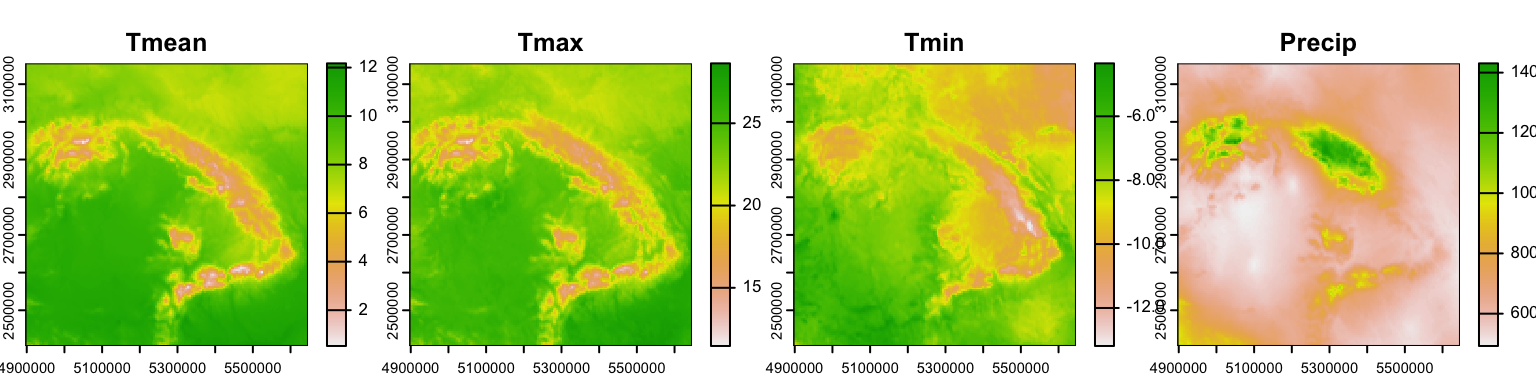
Alternatively, you can specify the numeric id’s of the layers you want to plot. The code below plots only layer 1.
plot(s, 1)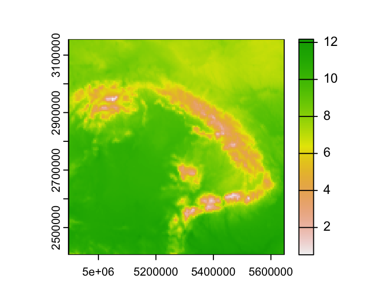
rasterVis
The rasterVis
package provides more flexible visualization routines. You may try them
out as well.
levelplot(s, layers=1)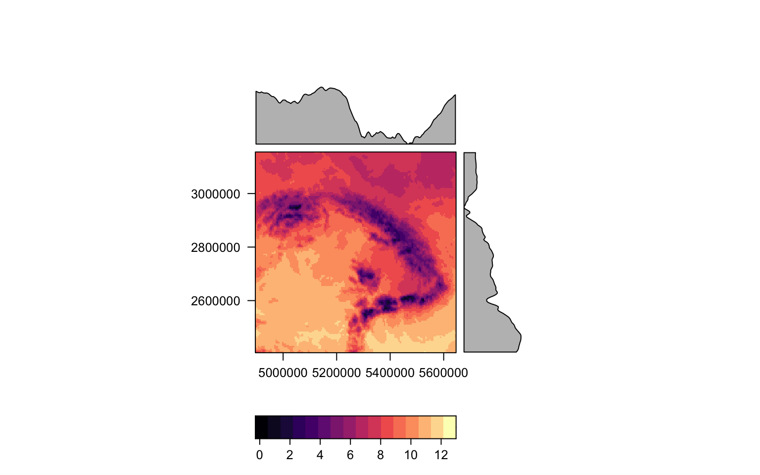
Write SpatRaster
Use writeRaster to write raster data. You must provide a SpatRaster and a filename. The file format will be guessed from the filename extension. If that does not work you can provide an argument like format=GTiff. Note the argument overwrite=TRUE and see ?writeRaster for more arguments, such as datatype= to set the a specific datatype (e.g., integer).
x <- writeRaster(r, "test_output.tif", overwrite=TRUE)
x
Sampling
Raster can have millions of pixels, which can make computations very
slow. So, sometimes it is useful to do calculations only on a sample of
the raster pixels, e.g. for estimating mean and standard deviation of a
raster, for building a statistical model. The spatSample
function can be used to extract a random sample in different ways. For
example, the random sample specified below yields a data.frame. If you
want to retrieve the same random sample every time you re-run
spatSample, set the random seed to the same number. This is helpful when
debugging your code, and you want to exclude random variations during
your testing.
set.seed(42)
df <- spatSample(s, size=1000, method="random")
head(df)
## Tmean Tmax Tmin Precip
## 1 9.597917 22.42300 -5.403000 895.7500
## 2 10.862667 25.25700 -5.679000 673.5000
## 3 9.392083 24.67600 -8.257000 549.2500
## 4 8.151889 22.26733 -8.205333 556.6667
## 5 10.574889 25.52800 -7.461333 562.1667
## 6 8.126028 22.29333 -8.400666 584.8333You can also return a SpatVector object.
set.seed(42)
sv <- spatSample(s, size=1000, method="random", as.points=T, as.df=F)
..or even a raster object when sampling in regular intervals.
set.seed(42)
sr <- spatSample(s, size=1000, method="regular", as.raster=T, as.df=F)
plot(sr, 1:2)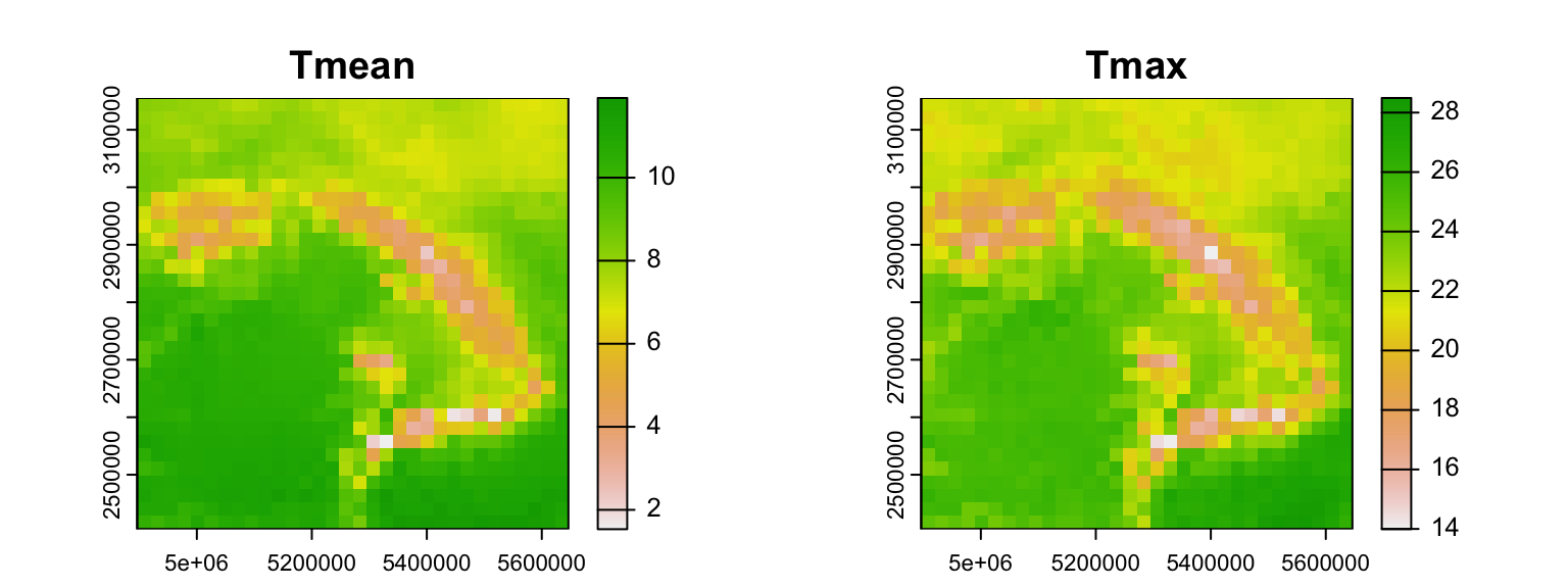
Predict
The terra package has two functions to make model
predictions to (potentially very large) rasters. The function
predict takes a multilayer raster and a fitted model as
arguments. Fitted models can be of various classes, including lm, glm,
gam, RandomForest, and prcomp (PCA). We’ve used predict already to apply
linear models to data.frames. The function interpolate is
similar but is for models that use coordinates as predictor variables,
for example in Kriging and spline interpolation. Type this into the
console to see the corresponding help page.
?`predict,SpatRaster-method`Copyright © 2024 Humboldt-Universität zu Berlin. Department of Geography.
![]()