- Packages
- Data
- Convert ppp to sf
- Convert sf to ppp
- Geographic distribution
- Centroid
- Dispersion
- Distance methods
- Pairwise distance
- Nearest neighbor distance
- G-Function
- K-Function
- Density methods
- Quadrat Count
- Kernel estimation
- Kernel maps with ggplot2
- Reading
Point Pattern Analysis
Humboldt-Universität zu Berlin | Geography Department
Packages
library(terra)     # Reading and manipulating raster data
library(sf)        # Reading and manipulating vector data
library(dplyr)     # Manipulating data.frames
library(ggplot2)   # Visualization
library(spatstat)  # Point Pattern Analysis
library(spatialEco) # Kernel density estimation
library(MASS)      # Bandwidth estimation for kernel density estimation
The package spatstat supports a wide range of popular
techniques for statistical analysis for spatial point patterns, for
example
- kernel estimation of density/intensity
- quadrat counting and clustering indices
- detection of clustering using Ripley’s K-function
- spatial logistic regression
- model-fitting
- Monte Carlo tests
Data
We are going to use the nbfires dataset built-in the
spatstat package. The dataset nbfires represents
point patterns created from yearly records of all fires between 1987 and
2003 falling under the jurisdiction of the New Brunswick Department of
Natural Resources. The dataset includes the boundary of the study area
(window), the point locations, and the following attributes
(marks) (see ?nbires):
year: This a factor with levels 1987, 1989, …, 2002, 2003. Note that 1988 is not present in the levels.
fire.type: A factor with levels forest, grass, dump, and other.
dis.date: The discovery date of the fire, which is the nearest possible surrogate for the starting time of the fire.
dis.julian: The discovery date and time of the fire, expressed in ‘Julian days’, i.e. as a decimal fraction representing the number of days since the beginning of the year (midnight 31 December).
cause: General cause of the fire.
fnl.size: The final size of the fire (area burned) in hectares, to the nearest 10th hectare.
Once you load the package, you can access the dataset as follows.
data("nbfires")
class(nbfires)
## [1] "ppp"Convert ppp to sf
The dataset is of class ppp (point pattern dataset). To
be able to work with the data outside the spatstat package,
we will convert it to a spatial data.frame (sf) as
follows.
# rescale to original units (km)
nbfires <- spatstat.geom::rescale(nbfires)

# remove fires with zero burned areas
nbfires <- subset(nbfires, fnl.size > 0)

# grab boundary polygon
boundary <- st_as_sf(nbfires$window, crs=2953)
st_crs(boundary) <- sf::st_crs('EPSG:2953')

# extract coordinates and attributes (marks) into a data.frame
df.fires <- data.frame(x=nbfires$x, y=nbfires$y, marks(nbfires))

# create spatial data.frame of fire locations
fires <- st_as_sf(df.fires, coords=c("x", "y"), crs=2953)

# convert year from factor to numeric
df.fires$year <- as.numeric(as.character(df.fires$year))

head(fires)
## Simple feature collection with 6 features and 9 fields
## Geometry type: POINT
## Dimension: XY
## Bounding box: xmin: 241.3276 ymin: 239.8376 xmax: 307.4978 ymax: 314.1635
## Projected CRS: NAD83(CSRS) / New Brunswick Stereographic
## year fire.type dis.date dis.julian out.date out.julian cause ign.src
## 1 2000 forest 2000-05-04 19:15:00 124.76042 2000-05-05 12:00:00 125.45833 resid burn.w.perm
## 2 2000 forest 2000-04-18 14:00:00 108.54167 2000-04-18 19:00:00 108.75000 misc cigs
## 3 2000 grass 2000-05-03 16:30:00 123.64583 2000-05-03 18:00:00 123.70833 resid burn.no.perm
## 4 2000 forest 2000-05-03 16:10:00 123.63194 2000-05-03 16:48:00 123.65833 unknown unknown
## 5 2000 grass 2000-04-19 13:00:00 109.50000 2000-04-19 15:00:00 109.58333 unknown unknown
## 6 2000 forest 2000-04-07 12:00:00 97.45833 2000-04-07 13:45:00 97.53125 resid presc.burn
## fnl.size geometry
## 1 1.6 POINT (307.4978 314.1635)
## 2 7.0 POINT (264.0312 270.9045)
## 3 1.0 POINT (255.3652 252.2977)
## 4 0.1 POINT (241.3276 261.4233)
## 5 0.5 POINT (257.9639 246.7722)
## 6 2.0 POINT (292.3899 239.8376)Convert sf to ppp
Functions from the spatstat package require spatial
objects of class ppp. We can create a ppp
object with the as.ppp() function, which takes a set of
coordinates and the bounding box (window).
fires_1999 <- as.ppp(st_coordinates(fires), st_bbox(fires))Geographic distribution
Centrographic statistics are tools used to analyze geographic distributions by measuring the center, dispersion and directional trend of a spatial arrangement (Grekousis, 2020).
Centroid
There are several ways to describe the centroid or center of the
geographic distribution. The mean center can easily be
calculated by averaging the coordinates. We can use the
summarize() function from the dplyr package to
calculate the mean x and y coordinate.
centroid <- summarize(df.fires,
                      x = mean(x),
                      y = mean(x))

ggplot(centroid) +
  geom_point(size=2, aes(x = x, y = y)) +
  geom_point(data=df.fires, aes(x=x, y=y), alpha=0.01) +
  coord_fixed() +
  geom_sf(data=boundary, aes(), fill=NA)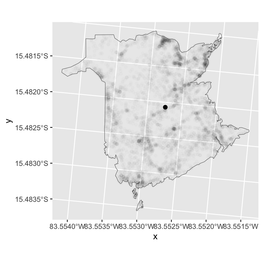
The figure above shows all fire locations in the background (high
transparency) and the overall mean represented by the bold point. The
overall mean location is not very meaningful. What is often done, is to
see how the geographic center of the distribution changes over time or
with different factors. Use the group_by() function to
calculate the mean by year (see Lab 3 for data manipulation with
dplyr).
centroids <- df.fires %>%
  group_by(year) %>%
  summarize(x = mean(x),
            y = mean(y))

ggplot(centroids) +
  geom_point(size=2, aes(x = x, y = y, col=year)) +
  geom_point(data=df.fires, aes(x=x, y=y), alpha=0.01) +
  coord_fixed() +
  geom_sf(data=boundary, aes(), fill=NA)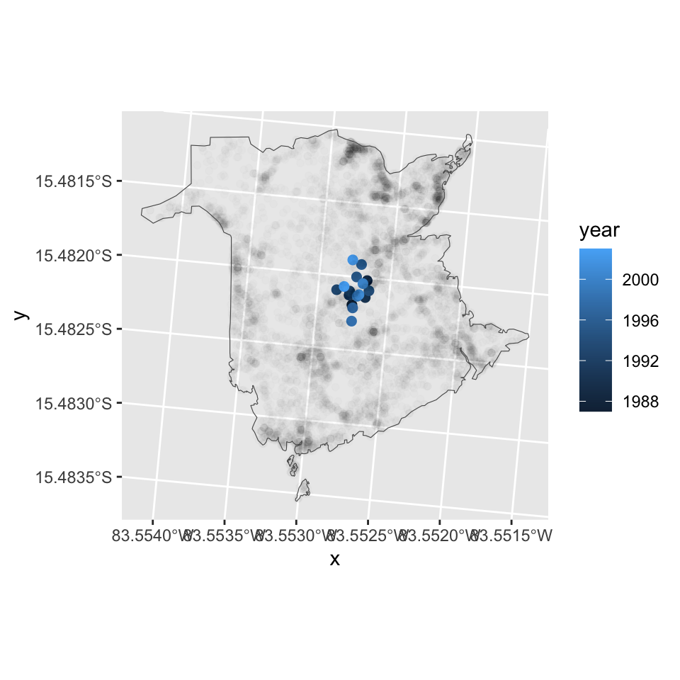
Fires actually do not represent points but areas, and those areas can vary substantially. To account for the burned area size, we can calculated a weighted average. The results show that the geographic distribution of the fires was more skewed/peripheral in the 1990s then in the 2000s when burned area size is accounted for.
centroids.w <- df.fires %>%
  group_by(year) %>%
  summarize(x = weighted.mean(x, w=fnl.size),
            y = weighted.mean(y, w=fnl.size))

ggplot(centroids.w) +
  geom_point(size=2, aes(x = x, y = y, col=year)) +
  geom_point(data=df.fires, aes(x=x, y=y), alpha=0.01) +
  coord_fixed() +
  geom_sf(data=boundary, aes(), fill=NA)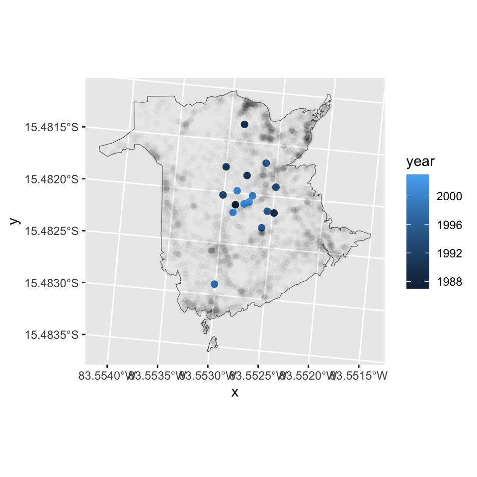
Dispersion
The dispersion or spread of the geographic distribution can be
described with the standard distance (circle) or (better) Standard
deviational ellipses. Standard deviational ellipse is calculated from
standard distance separately in the x and y direction. The feature is
available in ArcGIS, QGIS, and recently in the sfdep in R
package. Alternatively, ggplot can be used to fit and visualize ellipses
using a multi-normal distribution.
ggplot(df.fires) +
  geom_point(aes(x = x, y = y), alpha=0.01) +
  geom_point(data=centroid, aes(x=x, y=y), color=4) +
  stat_ellipse(aes(x = x, y = y), type = "norm", level=0.68, color=4) +
  coord_fixed() +
  geom_sf(data=boundary, fill=NA)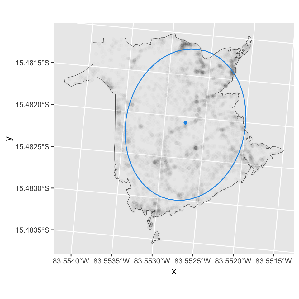
Distance methods
Distance-based methods of Point Pattern Analysis use the distances among events and describe second-order effects. Such methods include the nearest neighbor method, the G and F distance functions, the Ripley’s K distance function. There are different kinds of distances that can be measured in a point pattern (Baddeley et al., 2015):
pairwise distances s_{ij}=‖xi−xj‖ between all distinct pairs of points x_i and x_j (i≠j) in the pattern
nearest neighbor distances t_i=min_{j≠i}d_{ij}, the distance from each point x_i to its nearest neighbor
empty space distances d(u)=min_j‖u−x_i‖, the distance from a fixed reference location u in the window to the nearest data point
Since our dataset contains many locations that reburned over the
years, we will look at the point patterns of a single year only. With
the subset() function, we can select points based on the
values of their attributes/marks. Here, we select all fires of 1999,
which was one of the most fire-prone years in the time series.
fires_1999 <- subset(nbfires, year==1999)Pairwise distance
The pairwise distances can be calculated with the
pairdist() function of the spatstat package.
The result is a matrix of pairwise distances.
M <- pairdist(fires_1999)
M[1:5, 1:5]
## [,1] [,2] [,3] [,4] [,5]
## [1,] 0.00000 182.66553 185.52887 98.48238 106.50998
## [2,] 182.66553 0.00000 20.36504 102.87299 91.07527
## [3,] 185.52887 20.36504 0.00000 98.01737 86.47086
## [4,] 98.48238 102.87299 98.01737 0.00000 11.79779
## [5,] 106.50998 91.07527 86.47086 11.79779 0.00000We can look at the frequency distribution of the pairwise distances.
The square matrix contains the distances twice (point A to B and point B
to A) as well as the diagonal elements (distance of the points to
themselves). So, we extract only the distances of the upper triangle of
the matrix using upper.tri().
Mup <- M[upper.tri(M, diag=F)]
hist(Mup, xlab="Pairwise distance (km)", main="")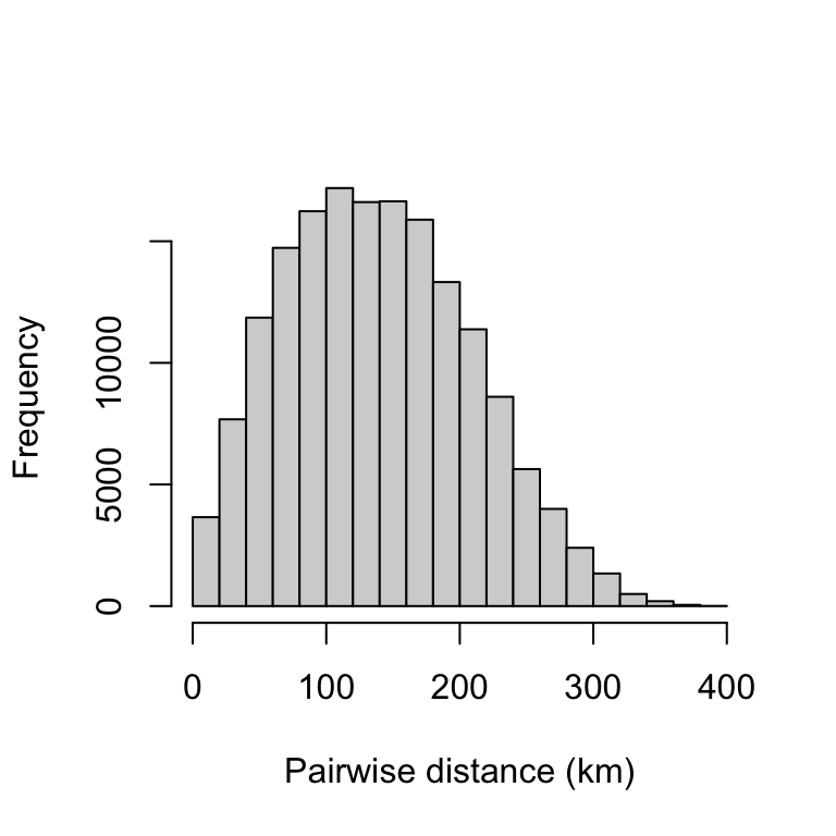
The mean pairwise distance is 139.06 km, and 50% of the data points are within 85.15 and 187.66 km apart.
summary(Mup)## Min. 1st Qu. Median Mean 3rd Qu. Max.
## 0.00 85.15 135.12 139.06 187.66 394.23Nearest neighbor distance
The nearest neighbor distances can be calculated with the
nndist() function of the spatstat package.
N <- nndist(fires_1999)
head(N)
## [1] 1.255376 2.234451 3.907304 2.230816 3.103236 3.908466The result is a vector with a length corresponding to the number of events. The heavily skewed frequency distribution below already indicates a spatially clustered distribution of the events.
hist(N, xlab="Nearest neighbor distance (km)", main="")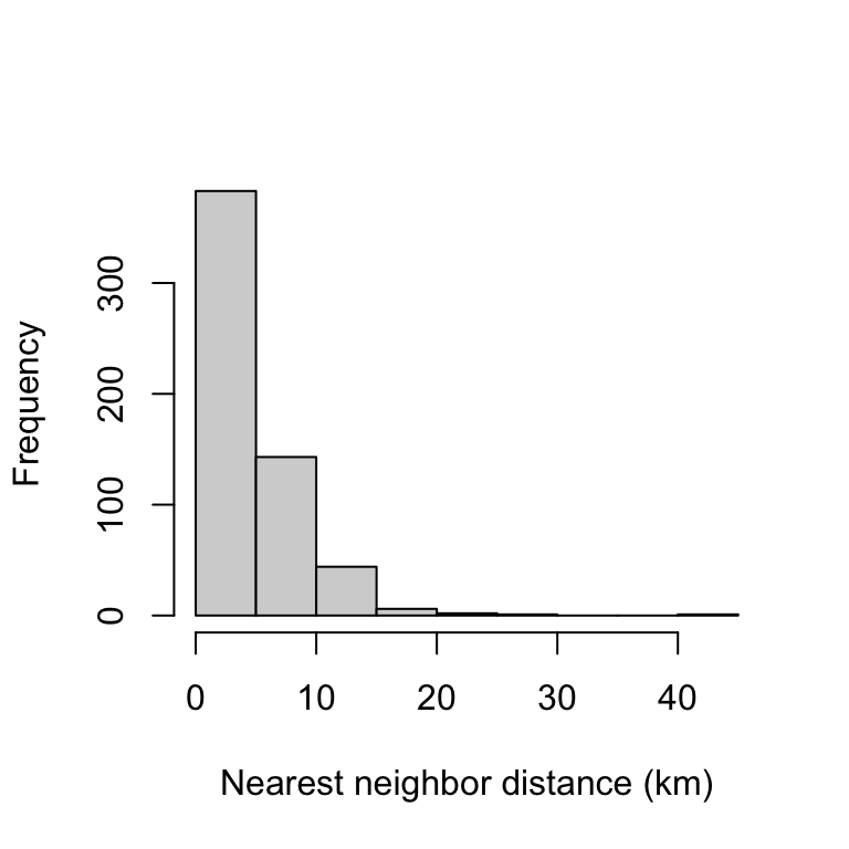
On average, the nearest neighbor was 4.44 km away, and 50% of the data points had neighbors that were less than 5.7 km away.
summary(N)## Min. 1st Qu. Median Mean 3rd Qu. Max.
## 0.000 1.851 3.702 4.440 5.702 41.506G-Function
The spatial arrangements of points can be described via the
cumulative distribution function of the nearest-neighbor distances, also
called the G-Function. The G-Function can be computed
from a point pattern object using the Gest() function. The
result of Gest is an object of class fv,
containing several estimates of the function using different edge
corrections, together with the theoretical value for a homogeneous
Poisson process with the same average intensity.
Gs <- Gest(fires_1999)
plot(Gs)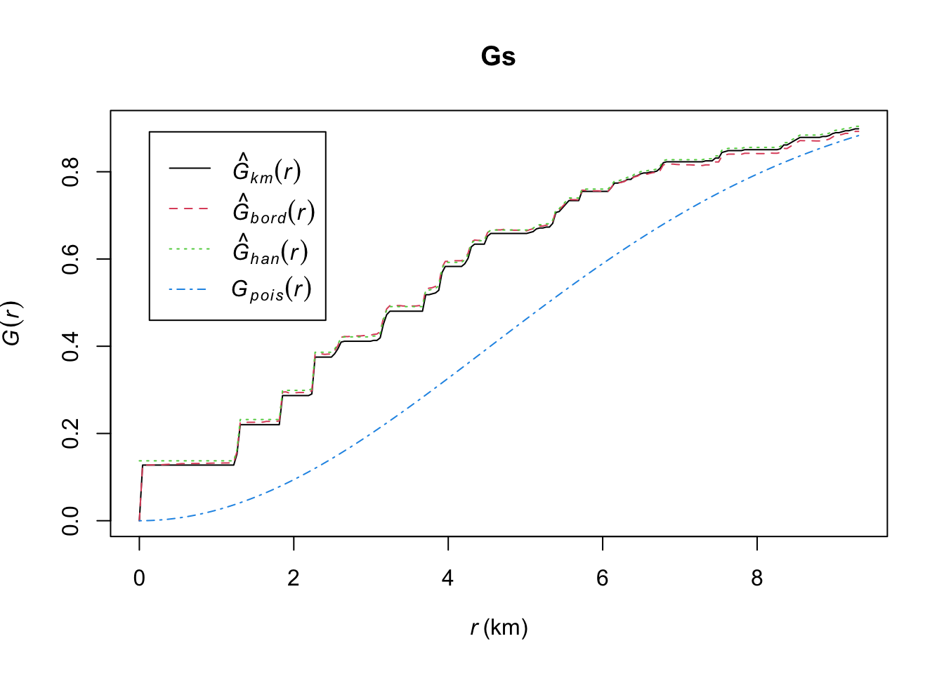
The plot shows three very similar estimates of the G Function and the theoretical function for complete spatial randomness. Also, the empirical curve lies above the theoretical curve for a completely random pattern, indicating that the nearest-neighbor distances in the data are shorter than expected for a completely random pattern. This is consistent with clustering.
Specifically, the curves shows that \hat{G}(r)=0.5 is achieved at about r=4, which means that 50% of the nearest-neighbor distances were 4 km and shorter.
K-Function
A very popular technique for analyzing spatial correlation in point
patterns is the K-function also known as Ripley’s K-function.
The empirical K-function Kb(r) is the cumulative average
number of data points lying within a distance r of a
typical data point, corrected for edge effects, and standardized by
dividing by the intensity. The standardization and edge correction make
it possible to compare point patterns with different numbers of points,
observed in different windows. The Kest() function of the
spatstat package provides several correction methods. By
default, Ripley’s isotropic correction (\hat{K}_{iso}), the border method (\hat{K}_{bord}), and the translation
correction (\hat{K}_{trans}) are
shown (see ?Kest for more info and references).
Ks <- Kest(fires_1999)
plot(Ks)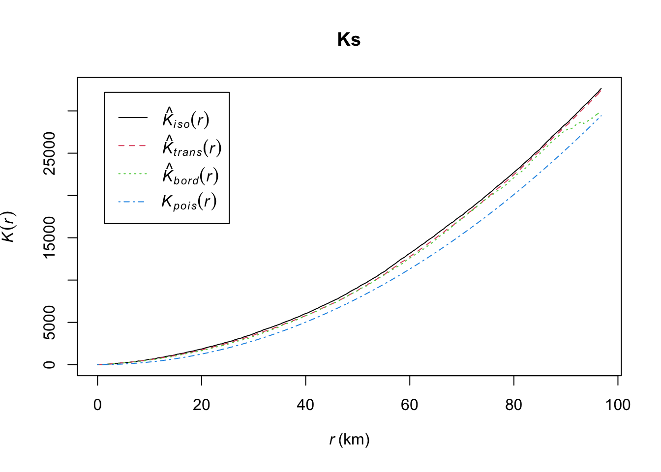
K values greater than expected K_{pois}(r) indicate clustering of points at a given distance band; K values less than expected K indicate dispersion of points at a given distance band. In our example, the fires appear to be more clustered than expected at all distances.
Density methods
Density-based methods of Point Pattern Analysis use the intensity of event occurrence across space and describe primarily first order effects.
Quadrat Count
A simple approach to measure intensity is by dividing the study area
into quadrats, and then counting the number of events in each quadrat.
We can do this using the spatstats package, but also using
the rasterize() function of the terra package.
The later has the advantage, that it produces a spatial raster that can
be exported/imported into other GIS/remote sensing software.
The rasterize() function requires a template raster as
input. The template raster can be an existing, valid raster or an empty
raster (no cell values). We can create an empty raster based on the
extent of the fires dataset.
extent <- ext(fires)
extent
## SpatExtent : 5.32663774943351, 399.060467986465, 2.21637329360078, 386.006349504711 (xmin, xmax, ymin, ymax)ras <- rast(extent)We also need to define the spatial resolution, here 10 x 10 km. This yields a raster with 38 rows and 39 columns:
res(ras) <- c(10, 10)
ras
## class : SpatRaster
## dimensions : 38, 39, 1 (nrow, ncol, nlyr)
## resolution : 10, 10 (x, y)
## extent : 5.326638, 395.3266, 2.216373, 382.2164 (xmin, xmax, ymin, ymax)
## coord. ref. :Next, we can use this raster as template to rasterize the points and
count the number of points in each cell. If you have an older version of
terra, you may need to convert the fires data (which is an
sf object) into a SpatVector object using the
vect() function. The argument fun takes either
the name of (some) built-in functions or a function object.
For simple functions like mean, max, length, etc, it is sufficient to
specify the name of the function in quotes. When rasterizing a spatial
point vector, all points falling in a raster grid cell are put into an
atomic R vector (non-spatial vector). The length of that vector
represents the count of the fires falling into that cell. The function
returns NA if there are no points inside a cell.
fire_count <- terra::rasterize(fires, ras, fun = "length", background = 0)
plot(fire_count)
plot(boundary, add=T)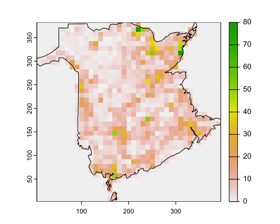
Here an example for using a function directly as input to the
rasterize function.
count_fires <- function(x) length(x)

fire_count <- terra::rasterize(fires, ras, fun=count_fires, background = 0)
Kernel estimation
Kernel density methods estimate the localized density (probability) of events based on a moving window. Unlike with the fixed quadrats the subregions overlap with the moving windows yielding smoother density surfaces. The shape and size of the moving window, as well as weights are defined by the Kernel function (e.g., Gaussian, quadratic).
The outcome of the Kernel estimation strongly depends on the Kernel
function and the bandwidth factor h. There are different ways to select an
appropriate value for h, but it is
important to note that there is a good deal of subjectivity involved.
Often h is determined by trial and
error and visual assessment of the output. Grekousis (2020) suggest the
use of Ripley’s K (or its
transformed L function) to set the bandwidth based on the clustering or
dispersion distances. Below, we use a simple algorithm to determine
bandwidth for Gaussian kernels from Venables and Ripley (2002). The
algorithm is available with the bandwidth.nrd() in the
MASS package.
bw_x <- bandwidth.nrd(df.fires$x)
bw_y <- bandwidth.nrd(df.fires$y)
c(bw_x, bw_y)
## [1] 54.83655 68.72043We can then calculate the Kernel density raster using
sp.kde() from the spatialEco package.
mapextent <- as.vector(ext(ras))
mapres <- res(ras)

fire_kde <- spatialEco::sf.kde(fires, bw = c(bw_x, bw_y), res = mapres,
                               ref = mapextent, standardize = T)
plot(fire_kde)
plot(boundary, add=T)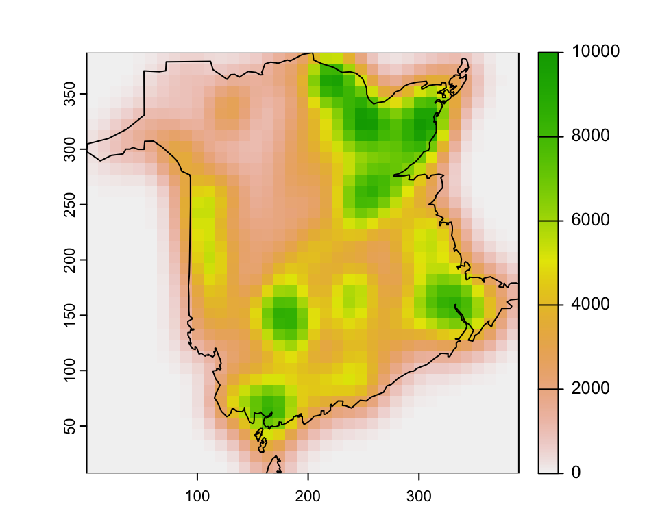
Kernel maps with ggplot2
The ggplot2 package also estimates kernel density maps (based on MASS::kde2d()).
ggplot() +
  stat_density2d(data = df.fires,
                 aes(x = x, y = y, fill = after_stat(level), alpha = after_stat(level)),
                 h=c(bw_x, bw_y), bins = 50, geom = "polygon") +
  scale_fill_gradient(low = "green", high = "red") +
  geom_density2d(data = df.fires, aes(x = x, y = y), linewidth = 0.1) +
  scale_alpha(range = c(0.1, 0.5), guide = 'none') +
  geom_sf(data=boundary, fill=NA)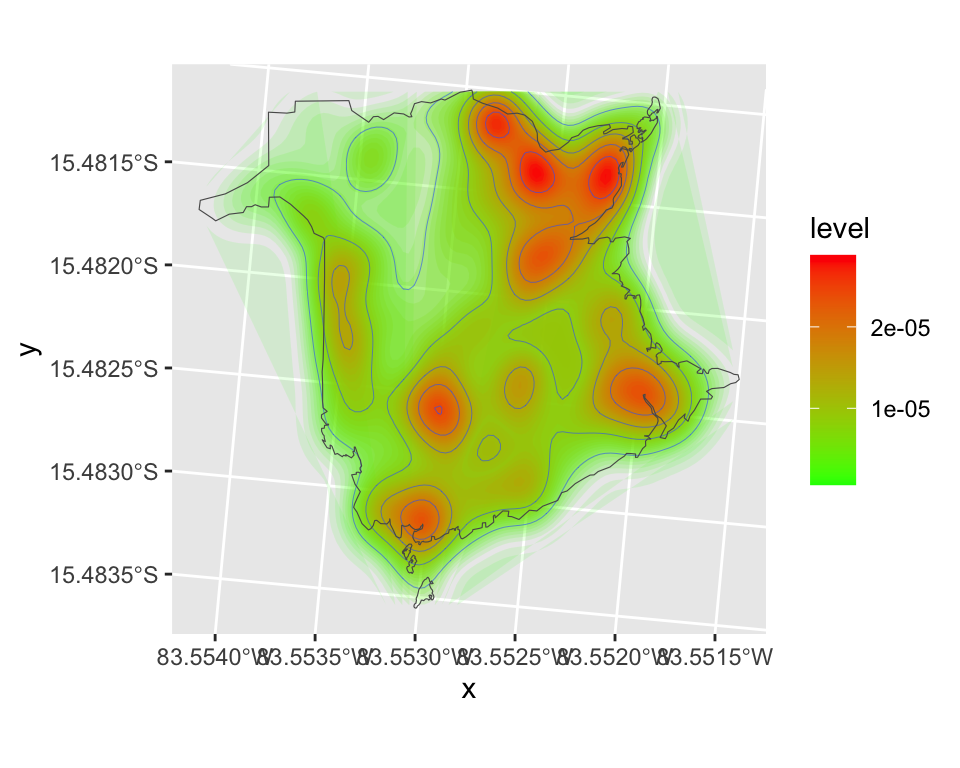
Reading
Venables, W. N. and Ripley, B. D. (2002) Modern Applied Statistics with S. Springer, equation (5.5) on page 130.
Copyright © 2024 Humboldt-Universität zu Berlin. Department of Geography.
![]()