- What is R?
- Getting R
- Install R
- R interface
- R interpreter
- RStudio
- Citing R
- The R language
- Syntax (Grammar)
- Expressions and assignments
- Comments
- Workspace
- Help
- Data types
- Integer and double
- Character
- Logical
- Missing values
- Type coercion
- Math operators and functions
- Logical operators
- Vectors
- Vectorized operations
- Recyling of vectors
- Statistical functions
- Logical vectors
- Generating vectors
- Sequences
- Repeats
- Numerical indexing
- Removing values of a vector
- Overwriting values of a vector
- Logical indexing
1. Introduction to R
Humboldt-Universität zu Berlin | Geography Department
What is R?
R is a statistical programming language that lets you:
- write functions
- analyze data
- apply most available statistical techniques
- create simple and complex graphs
- write your own library functions and algorithms
- process spatial data
- document your research and make it easier to reproduce
Furthermore, R is…
- Supported by a large user group
- Often compared to MatLab and Python
- Open source
- Can be linked to other languages (C, Fortran, Python, Stan, etc.)
Getting R
Install R
You can download R for Windows and other operating systems from the R Project Webpage. To install R on macOS and Linux, you may check out the How-To for macOS and Linux.
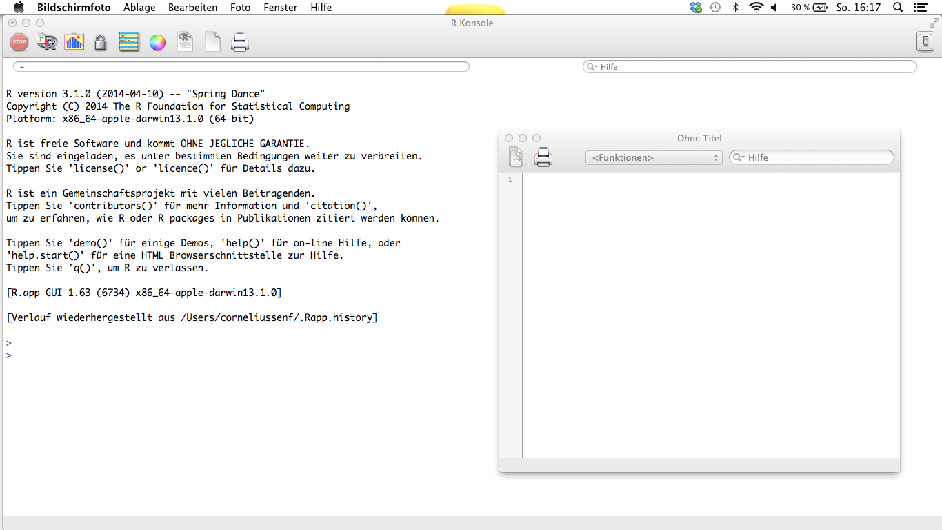
R interface
R ships with a console application (Windows) and a simple code editor.
R interpreter
- You need to write instructions (Code)
- R code follows a certain Syntax (Grammar)
- R Code is executed by the R interpreter
- R can interpret code:
- interactively in the Console (command-line)
- saved in a text file (Script) and sent entirely to the R interpreter
- Several IDE’s allow sending individual lines or entire scripts to the console
- Many outputs are displayed in the Console
- Graphical outputs are displayed in a separate window
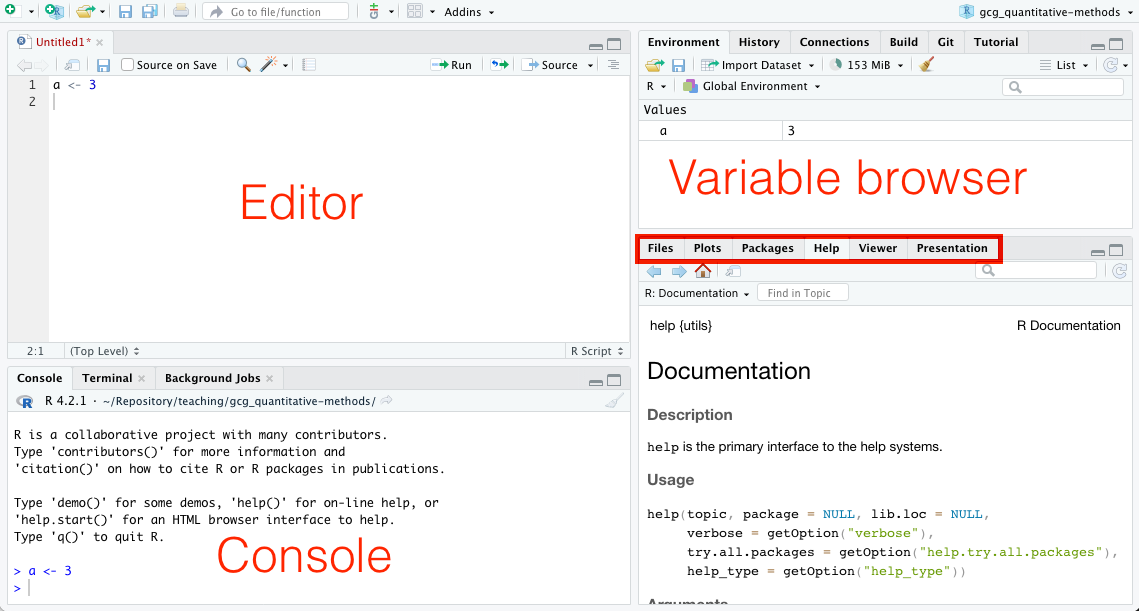
RStudio
RStudio is an Integrated Development Environment (IDE) that makes writing and interacting with R code easier. You can download RStudio here. Note, RStudio does include R. You need to install R along with RStudio. The RStudio Team has created some useful manuals to learn R and RStudio.
Citing R
citation()## To cite R in publications use:
##
## R Core Team (2024). _R: A Language and Environment for Statistical
## Computing_. R Foundation for Statistical Computing, Vienna, Austria.
## <https://www.R-project.org/>.
##
## A BibTeX entry for LaTeX users is
##
## @Manual{,
## title = {R: A Language and Environment for Statistical Computing},
## author = {{R Core Team}},
## organization = {R Foundation for Statistical Computing},
## address = {Vienna, Austria},
## year = {2024},
## url = {https://www.R-project.org/},
## }
##
## We have invested a lot of time and effort in creating R, please cite it
## when using it for data analysis. See also 'citation("pkgname")' for
## citing R packages.The R language
Syntax (Grammar)
- R is an expression language with a very simple syntax
- It is case sensitive, so A and a are different symbols and would refer to different variables
- All alphanumeric symbols are allowed as variable names plus ‘.’ and ‘_’
- However, a name must start with ‘.’ or a letter, and if it starts with ‘.’ the second character must not be a digit
- Names are effectively unlimited in length
Expressions and assignments
If an expression is given as a command, it is evaluated, printed (unless specifically made invisible), and the value is lost.
2 + 5## [1] 7An assignment also evaluates an expression and passes the value to a
variable but the result is not automatically printed. The assignment
operator is <- (“less than” and “minus”).
a <- 2 + 5If you enter the name of an existing variable into the console, its content is printed to the console output.
a## [1] 7If you assign a new expression to an already existing variable, this variable is overwritten.
b <- 5
a <- a + b
a
## [1] 12Workspace
The entities that R creates and manipulates are known as objects. These may be variables, arrays of numbers, character strings, and functions. The objects are stored in your current working environment (also called workspace). Once you quit an R session, these objects seize to exist. Note, the markdown documents that you use in the assignments run in their own workspace, which means a markdown document does not see the objects of your interactive workspace. This can sometimes lead to confusion when working interactively on assignments.
The function ls() can be used to display the names of
objects in your current workspace:
ls()## [1] "a" "b" "q"The function rm() can be used to remove objects from the
workspace:
rm(b)
ls()
## [1] "a" "q"It is possible to save and restore an entire workspace in R. However, I do not recommend this practice as you may loose track which objects are up-to-date ( with your code) and which are outdated. Instead, it is better to write reproducible code that easily lets you re-run and adapt your workflows.
Help
You can see the help for each R function using ?:
?is.nan()You can even get help for help:
?helpData types
Objects can store different types of data, i.e., not only numbers but
also text (character), logical (Boolean), and missing
values. You can use the function typeof() to identify the
data type.
Integer and double
The common numeric data types in R are integer and
double. An integer is a whole number (without decimal
places). A double is a real number. R treats many numeric values as
double by default, so that you do not have to worry about conversion or
loosing precision when doing integer division.
a <- 7
typeof(a)
## [1] "double"You can explicitly define an integer using a capital
L.
b <- 7L
typeof(b)
## [1] "integer"R automatically converts the result of the following integer division
to type double.
typeof(7L/2L)## [1] "double"7L/2L## [1] 3.5Character
d <- "hello world"
typeof(d)
## [1] "character"Combine two or more character variables with paste().
The default separator (sep) is whitespace.
paste("Hello", "World", sep = "_")## [1] "Hello_World"Extract a portion of a character variable
substring():
substring("Hello World", first = 3, last = 8)## [1] "llo Wo"Logical
The logical data type can have two possible values: TRUE
and FALSE. Both can be abbreviated as T and
F, respectively.
typeof(TRUE)## [1] "logical"Missing values
When an element or value is “not available” or a “missing value” in
the statistical sense, a place within a vector may be reserved for it by
assigning it the special value NA.
Any operation on an NA results in an NA
3 == NA## [1] NATo evaluate if a variable contains a missing value use
is.na():
is.na(3)## [1] FALSEThere is a second kind of “missing” values which are produced by
numerical computation, the so-called Not a Number, NaN,
values.
0 / 0## [1] NaNis.na() is TRUE both for NA
and NaN values. To differentiate these,
is.nan() is only TRUE for
NaNs.
Type coercion
R includes functions to set or change the data type:
as.character(a)## [1] "7"as.integer("3.1")## [1] 3as.double("3.1")## [1] 3.1Math operators and functions
There are several mathematical operators already implemented in R:
a <- 7
b <- 5
c <- a * b + sqrt(a) - b^2 / log(2) * 1.34 * exp(b)
c
## [1] -7135.204The elementary arithmetic operators are the usual +,
-, *, / and ^ for
raising to a power.
In addition all of the common arithmetic functions are available, e.g.:
sqrt(x): square root of xexp(x): antilog of x (e^x)log(x, n): log to base n of x (default n is e, natural log)log10(x): log to base 10 of xsin(x): sine of x in radianscos(x): cosine of x in radians- …and more
Logical operators
The logical data type can have TRUE and
FALSE values (and NA for not available).
The logical data type is a result of evaluating a condition, e.g. by using logical operators:
a == b # is a equal to b ?## [1] FALSEa < b # is a less than b ?## [1] FALSEa > b # is a greater than b ?## [1] TRUEThe %in% operator evaluates whether an element in the
first vector also part of the second vector. The operator returns a
logical vector of the same length as vector x.
x <- c(3, 9)
y <- c(1, 2, 3, 4, 5)
x %in% y
## [1] TRUE FALSEYou can combine logical operators (==,
<, <=, >,
>=, !=) or conditions with AND
(&) or OR (|):
a != b## [1] TRUEa != b & a < c## [1] FALSEa < b | a < c## [1] FALSEVectors
A vector is an ordered collection of values from a single data type.
Use c() to combine different values to a vector:
x <- c(1, 3, 8, 12, 56, 875, 234, 13)
x
## [1] 1 3 8 12 56 875 234 13Use length() to determine the number of values in a
vector:
length(x)## [1] 8You can construct vectors from each data type:
y <- c("a", "b", "c")
typeof(y)
## [1] "character"But you cannot mix data types. If you do, the simpler data type is used (coercion):
z <- c(1, 4, "b", 8.5, "abc")
typeof(z)
## [1] "character"The order is: Logical > Double > Integer > Character
Vectorized operations
To apply an arithmetic operation for each element of a vector, you
may be tempted to write a loop such as the one below. The example below
loops through each element i of vector x and
multiplies it with the number 2.
x## [1] 1 3 8 12 56 875 234 13for (i in x) {
i * 2
}However, this is not the way math is done in R. Most operations in
(base) R are vectorized, which means they are automatically performed
element by element. There is no need to loop over each element to do the
calculation. In fact, vectorization is better than looping. Loops in R
are relatively slow. The example below also applies the multiplication
and addition to each element of x. These operations are
vectorized.
x * 2## [1] 2 6 16 24 112 1750 468 26x + 2## [1] 3 5 10 14 58 877 236 15Vectorized operations also work between two vectors. In the following example, the first elements are added together, the second elements are added together, and so forth.
x <- c(1, 2, 3, 4, 5, 6, 7, 8)
y <- c(6, 3, 6, 9, 3, 1, 7, 2)
x + y
## [1] 7 5 9 13 8 7 14 10Recyling of vectors
If two vectors have different lengths, the shorter vector is recycled
(repeated) as often as needed to match the length of the longer vector.
In the example below, the y vector gets recycled four times
to c(1, 2, 1, 2, 1, 2, 1, 2).
x <- c(1, 2, 3, 4, 5, 6, 7, 8)
y <- c(1, 2)
x + y
## [1] 2 4 4 6 6 8 8 10Here, y gets recycled two time to
c(1, 5, 1, 3, 1, 5, 1, 3).
x <- c(1, 2, 3, 4, 5, 6, 7, 8)
y <- c(1, 5, 1, 3)
x + y
## [1] 2 7 4 7 6 11 8 11Recycling fails, if the length of y is not a multiple of
x.
x <- c(1, 2, 3, 4, 5, 6, 7, 8)
y <- c(1, 5, 3)
x + y
## Warning in x + y: longer object length is not a multiple of shorter object
## length## [1] 2 7 6 5 10 9 8 13Statistical functions
There are several functions that calculate a statistic from vectors such as:
max(): Maximummin(): Minimumsum(): Sum of all elementscumsum():Cumulative sum of all elementsprod(): Product of all elementssd(): Standard deviation of all elements
x## [1] 1 2 3 4 5 6 7 8sum(x)## [1] 36Recall that arithmetic operators applied to NA returns
NA. So, by default statistical functions return
NA when the vector contains even a single missing value.
This behavior is intentional. However, there is a way to have these
functions ignore NA values in their calculation using the
na.rm=TRUE keyword.
y <- c(1, 5, NA, 3)
sum(y)
## [1] NAsum(y, na.rm=TRUE)## [1] 9Logical vectors
x## [1] 1 2 3 4 5 6 7 8x < 4## [1] TRUE TRUE TRUE FALSE FALSE FALSE FALSE FALSEall(x < 4)## [1] FALSEany(x < 4)## [1] TRUEWhen arithmetic functions are applied to logical vectors,
TRUE is treated as the number 1 and
FALSE is treated as the number 0. This can be
very handy when counting the number of true values.
x## [1] 1 2 3 4 5 6 7 8sum(x < 4)## [1] 3Generating vectors
Sequences
R includes helpful functions for generating sequences:
1:10## [1] 1 2 3 4 5 6 7 8 9 1015:5## [1] 15 14 13 12 11 10 9 8 7 6 5seq(from = 1, to = 100, by = 10)## [1] 1 11 21 31 41 51 61 71 81 91Repeats
R includes helpful functions for generating repeats:
rep("x", times=10)## [1] "x" "x" "x" "x" "x" "x" "x" "x" "x" "x"rep(c("x", "o"), times=5)## [1] "x" "o" "x" "o" "x" "o" "x" "o" "x" "o"rep(c("x", "o"), each=5)## [1] "x" "x" "x" "x" "x" "o" "o" "o" "o" "o"Numerical indexing
You can access the ith value in a vector x
by using its positional index x[i]:
x <- c(1, 3, 8, 12, 56, 875, 234, 13)
x[1]
## [1] 1x[c(1, 5)]## [1] 1 56x[c(1:4, 8)]## [1] 1 3 8 12 13Removing values of a vector
You can remove values from a vector using negative indices:
length(x)## [1] 8x2 <- x[-3]
length(x2)## [1] 7Overwriting values of a vector
You can also overwrite individual values in a vector using indices.
Here, x[1] denotes the first element in x:
x[1] <- 5
x
## [1] 5 3 8 12 56 875 234 13Logical indexing
Instead of using a numeric index pointing to the ith
position of vector x, you can use a logical expression to
subset or extract elements of x that meet a certain
condition. For example, the expression below evaluations for every
element i in vector x if that element is
larger than 100. The result is a logical vector of TRUE and
FALSE that has the same length as x. If such a
logical vector is used as index vector all elements are extracted (or
replaced) where the index vector is TRUE.
x > 100## [1] FALSE FALSE FALSE FALSE FALSE TRUE TRUE FALSEx[x > 100]## [1] 875 234x[x > 100] <- 100
x## [1] 5 3 8 12 56 100 100 13Watch out. If the logical vector is shorter then x the
recycling rule applies!
x## [1] 5 3 8 12 56 100 100 13x[c(TRUE, FALSE)]## [1] 5 8 56 100x[c(TRUE, FALSE, TRUE)]## [1] 5 8 12 100 100Copyright © 2024 Humboldt-Universität zu Berlin. Department of Geography.
![]()
Comments
Comments start with a hash mark (
#). Everything that follows the hash mark up to the end of the line is ignored by the R interpreter. Comments can be entire lines or follow R code.# This is a comment b <- 5 # this also a <- a + b