Content

Multiple regression in R
Understanding interactions
Model-selection

Packages

library(MuMIn)   # exhaustive model selection
library(ggplot2)  # data visualization
library(effects) # extract model effects

Data

Let’s import the airquality dataset that we used in previous sessions.

# load airquality dataset
airq <- read.table("data/airquality.txt", sep = ",", dec = ".", header = TRUE)

# remove observations with missing data
airq <- na.omit(airq) 

# log-transform Ozone
airq$logOzone <- log(airq$Ozone)

# convert the numeric Month column into a factor variable
airq$Month <- factor(airq$Month, levels = 5:9,
                                 labels = c("May", "Jun", "Jul", "Aug", "Sep"))

# print first 5 rows of the dataset on screen
head(airq)

##   ID Ozone Solar Wind Temp Month Day logOzone
## 1  1    41   190  7.4   67   May   1 3.713572
## 2  2    36   118  8.0   72   May   2 3.583519
## 3  3    12   149 12.6   74   May   3 2.484907
## 4  4    18   313 11.5   62   May   4 2.890372
## 7  7    23   299  8.6   65   May   7 3.135494
## 8  8    19    99 13.8   59   May   8 2.944439

Exploratory analysis

Before constructing potentially complex linear models, it is important to visually explore your data and ask questions like:

What is the relationship between my response and predictor variables. Do I need to transform variables?
What is the relationship among my predictor variables? Do I need all? Do I need to account for collinearity?

You can evaluate the correlation between all variables by applying the cor() function to a data frame. With the methods argument, you can chose between the “pearson” (default), “kendall” and “spearman” correlation coefficients. Pearson measures linear correlation, while Kendall and Spearmann measure rank correlation and hence will pick up non-linear correlation.

cor(airq[, 1:4])

##                ID      Ozone       Solar       Wind
## ID     1.00000000  0.1375667 -0.08457572 -0.1803616
## Ozone  0.13756674  1.0000000  0.34834169 -0.6124966
## Solar -0.08457572  0.3483417  1.00000000 -0.1271835
## Wind  -0.18036162 -0.6124966 -0.12718345  1.0000000

You can obtain pairwise scatterplots between all the variables in the data set using the function pairs(). Note, package GGally provides the more sophisticated ggpairs() function.

pairs(airq[,1:4])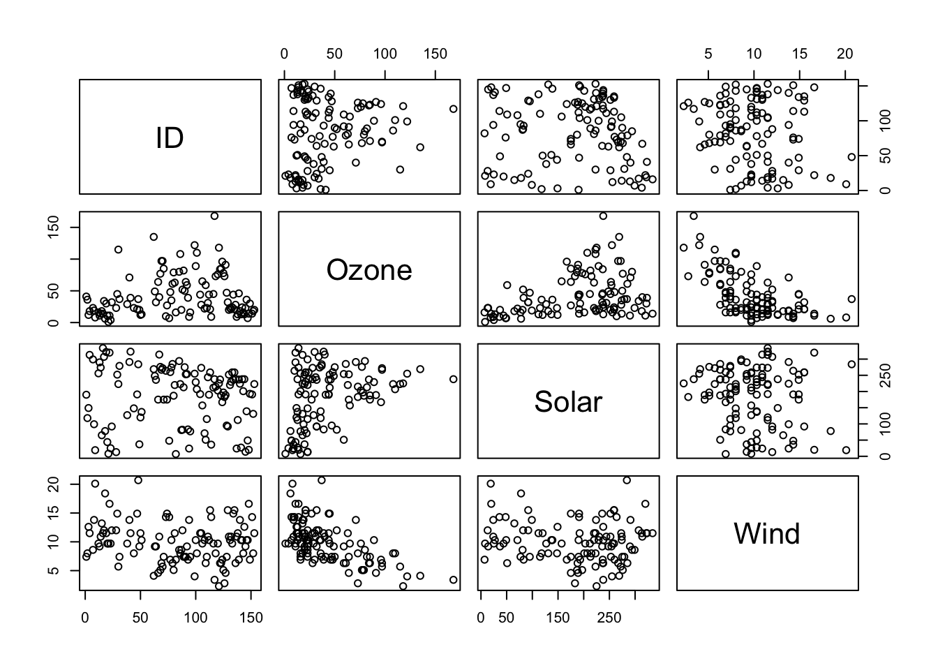

Multiple regression formula

Specification of a multiple regression analysis is done by setting up a model formula with + between the explanatory variables. The + means that we are constructing a model where the predictors have an additive effect on the response variable. Note, the intercept is explicitly included in this formula. We could include it explicitly by writing logOzone ~ 1 + Temp + Solar + Wind. If for some reason we wish to omit an intercept then we write logOzone ~ 0 + Temp + Solar + Wind.

lm1 <- lm(logOzone ~ Temp + Solar + Wind, data = airq)
lm1

## 
## Call:
## lm(formula = logOzone ~ Temp + Solar + Wind, data = airq)
## 
## Coefficients:
## (Intercept)         Temp        Solar         Wind  
##   -0.262132     0.049171     0.002515    -0.061562

We can add more complex terms, i.e. polynomials, “on-the-fly” using the I() function. The I() function “protects” the calculation inside the I() function call, such that operators like +, -, * and ^ are not misinterpreted as formula operators.

lm2 <- lm(logOzone ~ Temp + Solar + I(Solar^2) + Wind, data = airq)
lm2

## 
## Call:
## lm(formula = logOzone ~ Temp + Solar + I(Solar^2) + Wind, data = airq)
## 
## Coefficients:
## (Intercept)         Temp        Solar   I(Solar^2)         Wind  
##  -2.369e-01    4.492e-02    7.259e-03   -1.413e-05   -5.876e-02

You can use the update() function to add or remove predictors from a model:

# add a term from model lm2
lm3 <- update(lm2, . ~ . + I(Temp^2)) 
lm3

## 
## Call:
## lm(formula = logOzone ~ Temp + Solar + I(Solar^2) + Wind + I(Temp^2), 
##     data = airq)
## 
## Coefficients:
## (Intercept)         Temp        Solar   I(Solar^2)         Wind    I(Temp^2)  
##   3.932e+00   -6.687e-02    7.649e-03   -1.508e-05   -5.635e-02    7.280e-04

# remove a term from model lm3
lm4 <- update(lm3, . ~ . - Wind)
lm4

## 
## Call:
## lm(formula = logOzone ~ Temp + Solar + I(Solar^2) + I(Temp^2), 
##     data = airq)
## 
## Coefficients:
## (Intercept)         Temp        Solar   I(Solar^2)    I(Temp^2)  
##   3.561e+00   -8.328e-02    8.439e-03   -1.751e-05    8.983e-04

Dummy variables

A mathematical model can only work with numbers. So, how does R deal with categorical variables? Categorical predictor variables are internally recoded into multiple binary dummy variables, where each dummy variable switches a single factor level on (1) or off (0). For example, the variable Month in the airquality dataset has five factor levels: May, Jun, Jul, Aug, Sep. To illustrate the point, let’s recode the factor variable manually. Note, there are different names for dummy variables. Indicator variables is another common term.

airq$dummyJun <- ifelse(airq$Month=="Jun", 1, 0)
airq$dummyJul <- ifelse(airq$Month=="Jul", 1, 0)
airq$dummyAug <- ifelse(airq$Month=="Aug", 1, 0)
airq$dummySep <- ifelse(airq$Month=="Sep", 1, 0)

head(airq[!duplicated(airq$Month), -1])

##     Ozone Solar Wind Temp Month Day logOzone dummyJun dummyJul dummyAug dummySep
## 1      41   190  7.4   67   May   1 3.713572        0        0        0        0
## 38     29   127  9.7   82   Jun   7 3.367296        1        0        0        0
## 62    135   269  4.1   84   Jul   1 4.905275        0        1        0        0
## 93     39    83  6.9   81   Aug   1 3.663562        0        0        1        0
## 124    96   167  6.9   91   Sep   1 4.564348        0        0        0        1

We do not need to create a dummy for month May since month May is automatically coded when all other dummy variables are 0. So, if a variable has n factors, you need n-1 dummy variables. That also means the more factor levels the more parameters your model needs to estimate. Let’s build a linear regression model between logOzone and Temperature and Month using the dummy variables.

lm4 <- lm(logOzone ~ Temp + dummyJun + dummyJul + dummyAug + dummySep, data = airq)
summary(lm4)

## 
## Call:
## lm(formula = logOzone ~ Temp + dummyJun + dummyJul + dummyAug + 
##     dummySep, data = airq)
## 
## Residuals:
##      Min       1Q   Median       3Q      Max 
## -2.26925 -0.29321  0.03879  0.34206  1.50462 
## 
## Coefficients:
##              Estimate Std. Error t value Pr(>|t|)    
## (Intercept) -2.138938   0.546860  -3.911 0.000163 ***
## Temp         0.074715   0.008037   9.296 2.32e-15 ***
## dummyJun    -0.468759   0.243768  -1.923 0.057192 .  
## dummyJul    -0.244664   0.214692  -1.140 0.257045    
## dummyAug    -0.293629   0.217549  -1.350 0.180009    
## dummySep    -0.387591   0.179445  -2.160 0.033053 *  
## ---
## Signif. codes:  0 '***' 0.001 '**' 0.01 '*' 0.05 '.' 0.1 ' ' 1
## 
## Residual standard error: 0.5748 on 105 degrees of freedom
## Multiple R-squared:  0.5793, Adjusted R-squared:  0.5593 
## F-statistic: 28.92 on 5 and 105 DF,  p-value: < 2.2e-16

Now, as mentioned before, the dummy coding is actually done internally when you include a factor variable as predictor. You do not need to do the coding manually. So, before we discuss what the output means, let’s check out the ‘automated’ code version without manual dummy coding (recall, variable Month is a factor variable):

lm5 <- lm(logOzone ~ Temp + Month, data = airq)
summary(lm5)

## 
## Call:
## lm(formula = logOzone ~ Temp + Month, data = airq)
## 
## Residuals:
##      Min       1Q   Median       3Q      Max 
## -2.26925 -0.29321  0.03879  0.34206  1.50462 
## 
## Coefficients:
##              Estimate Std. Error t value Pr(>|t|)    
## (Intercept) -2.138938   0.546860  -3.911 0.000163 ***
## Temp         0.074715   0.008037   9.296 2.32e-15 ***
## MonthJun    -0.468759   0.243768  -1.923 0.057192 .  
## MonthJul    -0.244664   0.214692  -1.140 0.257045    
## MonthAug    -0.293629   0.217549  -1.350 0.180009    
## MonthSep    -0.387591   0.179445  -2.160 0.033053 *  
## ---
## Signif. codes:  0 '***' 0.001 '**' 0.01 '*' 0.05 '.' 0.1 ' ' 1
## 
## Residual standard error: 0.5748 on 105 degrees of freedom
## Multiple R-squared:  0.5793, Adjusted R-squared:  0.5593 
## F-statistic: 28.92 on 5 and 105 DF,  p-value: < 2.2e-16

The model results are the same as using manually coded dummy variables. You see the factor Month was recoded into dummy variables, though they are now named MonthJun, MonthJul, MonthAug, MonthSep. The first level (May) is automatically selected as the base level (e.g. if all other dummy variables are 0).

Variable intercept

With the previous model, we fitted a linear regression model using Temperature and Month as predictors. In other words, we let the linear relationship between Temperature and logOzone vary with Month. More precisely, we let only the intercept vary with Month. To illustrate how we can estimate the intercepts associated with the different levels of Month, we need to go back to our linear model equation:

\(logOzone = \beta_0 + \beta_1Temp + \beta_2MonthJun + \beta_3MonthJul + \beta_4MonthAug + \beta_5Sep + \epsilon\)

Since the dummy variables are binary, i.e. either 0 or 1, the equation above reduces to this equation for month May:

\(logOzone = \beta_0 + \beta_1Temp + \beta_2*0 + \beta_3*0 + \beta_4*0 + \beta_5*0\)

\(logOzone = \beta_0 + \beta_1Temp\)

… or for Month July:

\(logOzone = \beta_0 + \beta_1Temp + \beta_2*0 + \beta_3*1 + \beta_4*0 + \beta_5*0\)

\(logOzone = \beta_0 + \beta_1Temp + \beta_3\)

Since \(\beta_0\) and \(\beta_3\) are constants, we can rearrange as follows:

\(logOzone = (\beta_0 + \beta_3) + \beta_1Temp\)

To estimate the different intercepts, we replace the \(\beta's\) with the corresponding parameter outputs from summary(lm5), e.g. \(\beta_0\) is (Intercept), \(\beta_2\) is MonthJun, \(\beta_3\) is MonthJul, etc. For May the intercept of the regression line is \(\beta_0\) = -2.14 and for month July the intercept is \(\beta_0+\beta_3\) = -2.14 + -0.24 = -2.38 (for month August \(\beta_0+\beta_4\), etc.).

Example

coef(lm5) # access model coefficients (beta's)

## (Intercept)        Temp    MonthJun    MonthJul    MonthAug    MonthSep 
## -2.13893784  0.07471496 -0.46875932 -0.24466375 -0.29362919 -0.38759055

lm5_intercept_May <- coef(lm5)['(Intercept)']
lm5_intercept_May

## (Intercept) 
##   -2.138938

lm5_intercept_Jul <- coef(lm5)['(Intercept)'] + coef(lm5)['MonthJul']
lm5_intercept_Jul

## (Intercept) 
##   -2.383602

lm5_slope <- coef(lm5)['Temp']
lm5_slope

##       Temp 
## 0.07471496

You see that the only parameter that changes with Month in our model is the intercept and we can calculate the intercepts based on \(\beta_0\) and the \(\beta\)’s from our dummy variables. Let’s plot the regression lines for May and July based on the calculated intercepts.

ggplot(airq, aes(x = Temp, y = logOzone)) + 
  geom_point(aes(col = Month)) +
  scale_color_manual(values = c("#E41A1C", "#377EB8", "#4DAF4A", "#984EA3", "#FF7F00")) +
  geom_abline(slope=lm5_slope, intercept=lm5_intercept_May, col="#E41A1C") +
  geom_abline(slope=lm5_slope, intercept=lm5_intercept_Jul, col="#4DAF4A")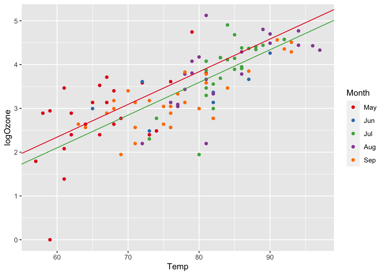

Interaction terms

So far, we only included an additive effect of Month, i.e. we allowed only the intercept to vary with Month. However, what if the effect is not additive? In other words, what if the effect of Month on Ozone is not constant? Perhaps, the effect of Month varies also with Temperature (or the other way round), in which case we need to let the slope vary with Month as well, not just the intercept. To include such interactions between predictor variables, we can include interaction terms.

In model formulas in R, interaction terms are generated using the colon operator: var1:var2.

Usually, the interaction term is included in addition to the additive effect:

respone ~ var1+var2 + var1:var2

Rather than writing both terms, you can use the shorthand: var1*var2. Hence, the following formula describes the same model as the formula above:

respone ~ var1*var2

Let’s try out an interaction between Temperature and Month with our airquality dataset.

lm6 <- lm(logOzone ~ Temp * Month, data = airq)
summary(lm6)

## 
## Call:
## lm(formula = logOzone ~ Temp * Month, data = airq)
## 
## Residuals:
##      Min       1Q   Median       3Q      Max 
## -2.19906 -0.26980  0.00246  0.35058  1.51166 
## 
## Coefficients:
##               Estimate Std. Error t value Pr(>|t|)    
## (Intercept)   -2.76430    1.19238  -2.318   0.0224 *  
## Temp           0.08413    0.01786   4.711 7.89e-06 ***
## MonthJun       2.42798    2.33970   1.038   0.3019    
## MonthJul      -3.95983    2.45826  -1.611   0.1103    
## MonthAug       0.11327    1.87091   0.061   0.9518    
## MonthSep       1.13404    1.54120   0.736   0.4635    
## Temp:MonthJun -0.03845    0.03123  -1.231   0.2211    
## Temp:MonthJul  0.04233    0.03121   1.357   0.1779    
## Temp:MonthAug -0.00680    0.02477  -0.275   0.7843    
## Temp:MonthSep -0.02107    0.02187  -0.963   0.3377    
## ---
## Signif. codes:  0 '***' 0.001 '**' 0.01 '*' 0.05 '.' 0.1 ' ' 1
## 
## Residual standard error: 0.568 on 101 degrees of freedom
## Multiple R-squared:  0.6048, Adjusted R-squared:  0.5696 
## F-statistic: 17.18 on 9 and 101 DF,  p-value: < 2.2e-16

The model output shows the parameter estimates for the base intercept, the additive effects of Temp and Month (coded as dummy variables), and the interaction terms with the colon sign (:).

Estimate interaction effects

To estimate how the slopes vary with Month, we need to go back to our model formula and combine the parameters as we did when estimating the intercepts from the additive dummy model. The parameters for the interaction terms are \(\beta_6\)-\(\beta_9\).

\(logOzone = \beta_0 + \beta_1*Temp + \beta_2*Jun + \beta_3*Jul + ... + \beta_5*Sep + \beta_6*Temp*Jun + \beta_7*Temp*Jul + ... + \beta_9*Temp*Sep\)

So, if we are interested in the relationship between Temperature and logOzone for May, the above equation reduces to:

\(logOzone = \beta_0 + \beta_1Temp\)

As May is our base factor level, all other \(\beta\)s get multiplied by zeros and therefore eliminated. The intercept of month May is \(\beta_0\) and the slope is \(\beta_1\).

If we are interested in the relationship between Temperature and Ozone for July (or some other month), the equation reduces as follows, where \(\beta_3\) estimates the additive term and \(\beta_6\) estimates the interaction term. Note, unlike in an R formula, where the \(*\) sign symbolizes the inclusion of both, additive and interaction terms, here \(*\) truly represents the multiplicative sign.

\(logOzone = \beta_0 + \beta_1Temp + \beta_3Jul + \beta_7*Temp*Jul\)

which we can rearrange as follows:

\(logOzone = (\beta_0 + \beta_3) + (\beta_1 + \beta_7)*Temp\)

where the intercept is \((\beta_0 + \beta_3)\) and the slope is \((\beta_1 + \beta_7)\).

Example

The coefficients of our airquality model with interaction term are as follows:

coef(lm6) # access model coefficients (beta's)

##   (Intercept)          Temp      MonthJun      MonthJul      MonthAug      MonthSep Temp:MonthJun 
##  -2.764304030   0.084124863   2.427979206  -3.959831889   0.113272053   1.134041099  -0.038447329 
## Temp:MonthJul Temp:MonthAug Temp:MonthSep 
##   0.042334206  -0.006799668  -0.021065369

To estimate ozone concentration for month May, we grab the intercept and slope term:

\(logOzone_{May} = -2.76 + 0.08 * Temp\)

To estimate ozone concentration for month July, we have to add the parameters for the July intercept offset (-3.96) and the slope offset from the interaction term (0.04):

\(logOzone_{July} = (-2.76 - 3.96) + (0.08 + 0.04) * Temp\)

We can do this directly in R and plot the corresponding regression lines:

lm6_intercept_May <- coef(lm6)['(Intercept)']
lm6_intercept_Jul <- coef(lm6)['(Intercept)'] + coef(lm6)['MonthJul']
lm6_slope_May <- coef(lm6)['Temp']
lm6_slope_Jul <- coef(lm6)['Temp'] + coef(lm6)['Temp:MonthJul']

ggplot(airq, aes(x = Temp, y = logOzone)) +
  geom_point(aes(col = Month)) +
  scale_color_manual(values = c("#E41A1C", "#377EB8", "#4DAF4A", "#984EA3", "#FF7F00")) +
  geom_abline(slope=lm6_slope_May, intercept=lm6_intercept_May, col="#E41A1C") +
  geom_abline(slope=lm6_slope_Jul, intercept=lm6_intercept_Jul, col="#4DAF4A")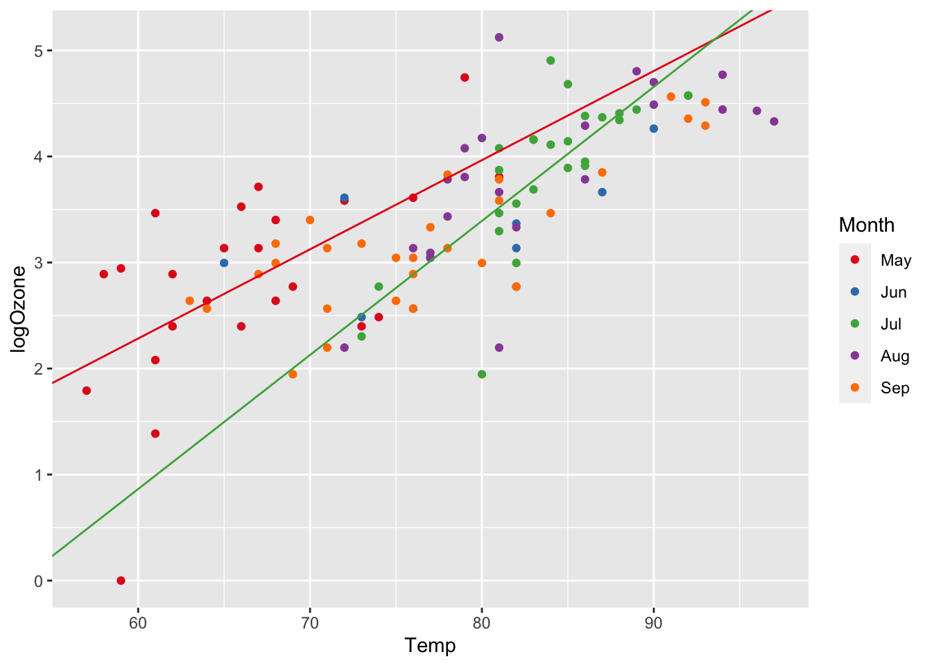

The `effects` package

As always, there already exists a package doing all the hard coding-work for us. In this case, we make use of the effect() function from the effects package:

efct <- effects::effect(term = "Temp:Month", mod = lm6)
efct <- as.data.frame(efct) # convert list to data.frame
efct$Month <- factor(efct$Month, levels = c("May", "Jun", "Jul", "Aug", "Sep"))
head(efct)

##   Temp Month      fit        se    lower    upper
## 1   60   May 2.283188 0.1635384 1.958772 2.607604
## 2   70   May 3.124436 0.1320779 2.862429 3.386443
## 3   80   May 3.965685 0.2681741 3.433700 4.497670
## 4   90   May 4.806934 0.4360770 3.941874 5.671993
## 5  100   May 5.648182 0.6100672 4.437973 6.858392
## 6   60   Jun 2.404327 0.5038101 1.404903 3.403751

Note: confidence intervals are calculated automatically. You can change the level of the confidence intervals setting the argument confint. See ?effect.

Plotting the regression on the log-scale:

ggplot(airq) +
  geom_point(aes(x = Temp, y = logOzone, col = Month)) +
  geom_line(data = efct, aes(x = Temp, y = fit, col = Month)) +
  scale_color_manual(values = c("#E41A1C", "#377EB8", "#4DAF4A", "#984EA3", "#FF7F00"))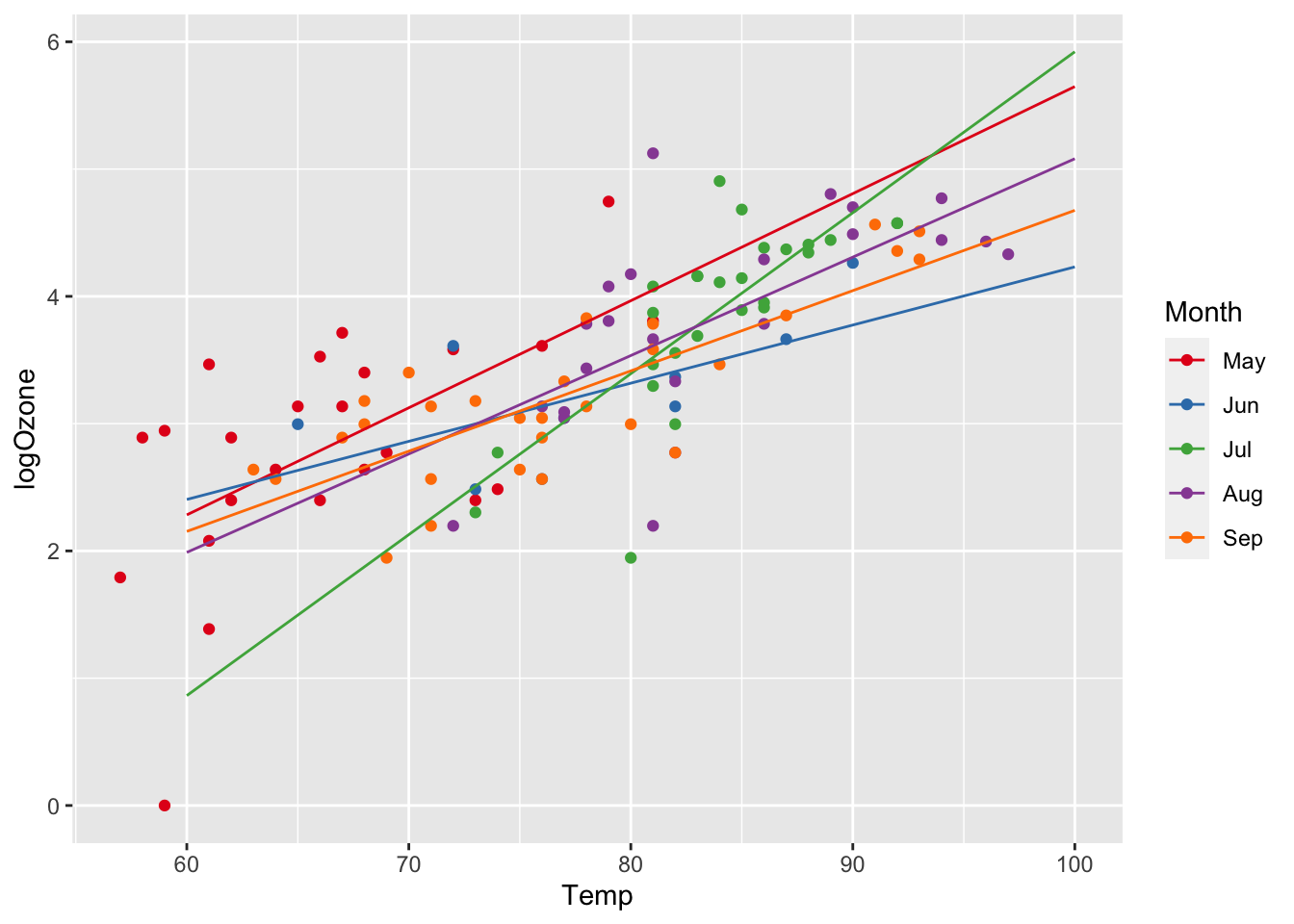

Add confidence intervals to the plot as ribbons using geom_ribbon():

ggplot(airq) +
  geom_point(aes(x = Temp, y = logOzone, col = Month)) +
  geom_ribbon(data = efct, aes(x = Temp, ymin = lower, ymax = upper, fill = Month), alpha = 0.2) +
  geom_line(data = efct, aes(x = Temp, y = fit, col = Month)) +
  scale_color_manual(values = c("#E41A1C", "#377EB8", "#4DAF4A", "#984EA3", "#FF7F00")) +
  scale_fill_manual(values = c("#E41A1C", "#377EB8", "#4DAF4A", "#984EA3", "#FF7F00"))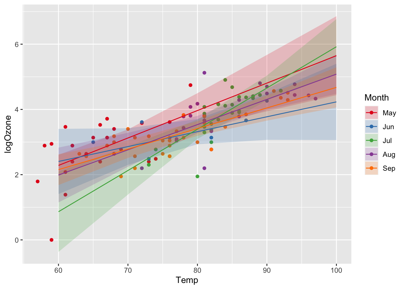

Converting predictions back to the linear scale:

efct <- effect(term = "Temp:Month", mod = lm6) 
efct <- as.data.frame(efct)
efct$Month <- factor(efct$Month, levels = c("May", "Jun", "Jul", "Aug", "Sep"))

ggplot(airq, aes(x = Temp, y = Ozone, col = Month)) +
  geom_point() +
  scale_color_manual(values = c("#E41A1C", "#377EB8", "#4DAF4A", "#984EA3", "#FF7F00")) +
  geom_line(data = efct, aes(y = exp(fit)))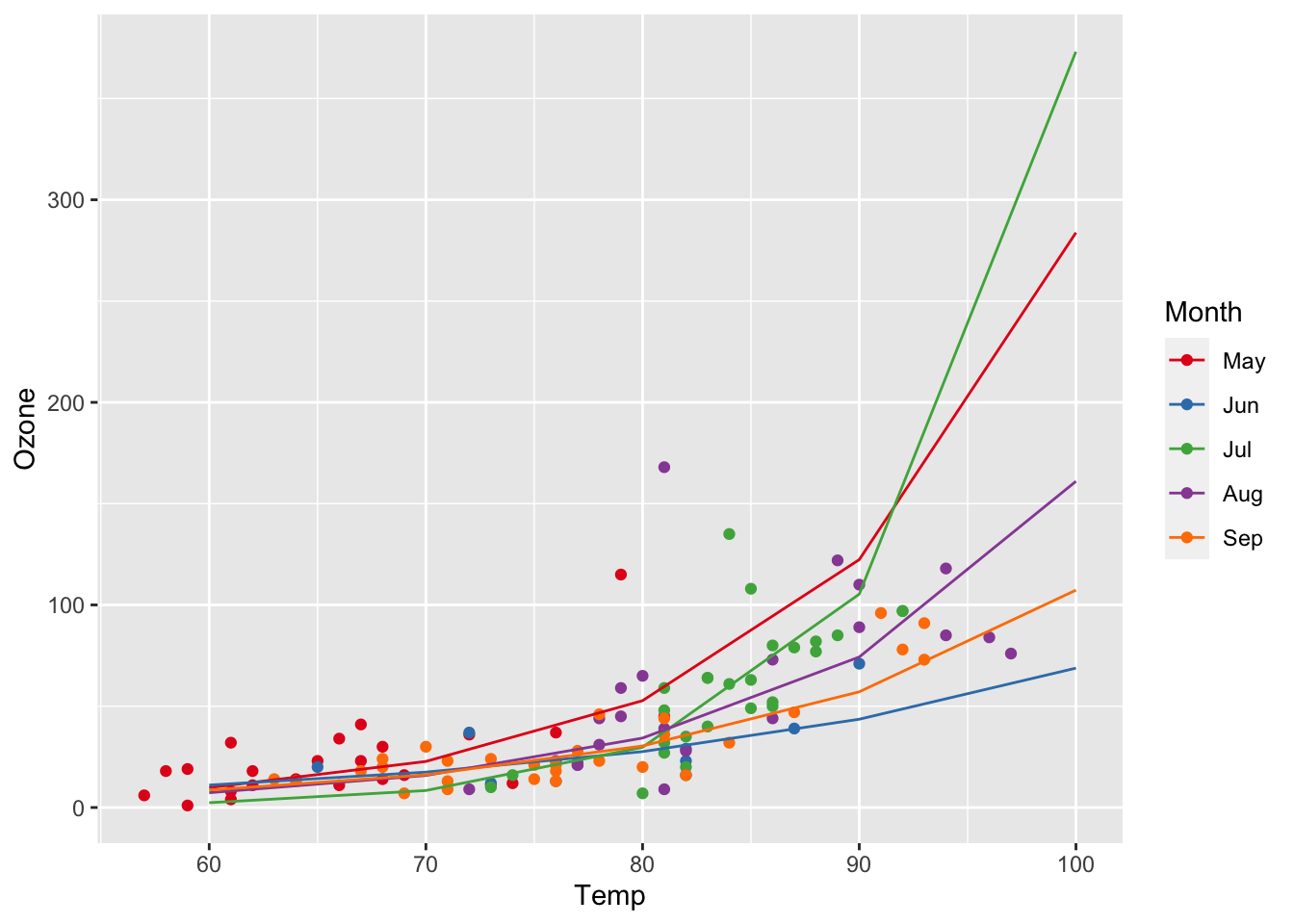

Resolving the simulation interval finer:

efct <- effect(term = "Temp:Month", mod = lm6, 
               xlevels = list(Temp = seq(57, 97, length.out = 100))) # Changing the x-levels
efct <- as.data.frame(efct)
efct$Month <- factor(efct$Month, levels = c("May", "Jun", "Jul", "Aug", "Sep"))

ggplot(airq, aes(x = Temp, y = Ozone, col = Month)) +
  geom_point() +
  scale_color_manual(values = c("#E41A1C", "#377EB8", "#4DAF4A", "#984EA3", "#FF7F00")) +
  geom_line(data = efct, aes(y = exp(fit)))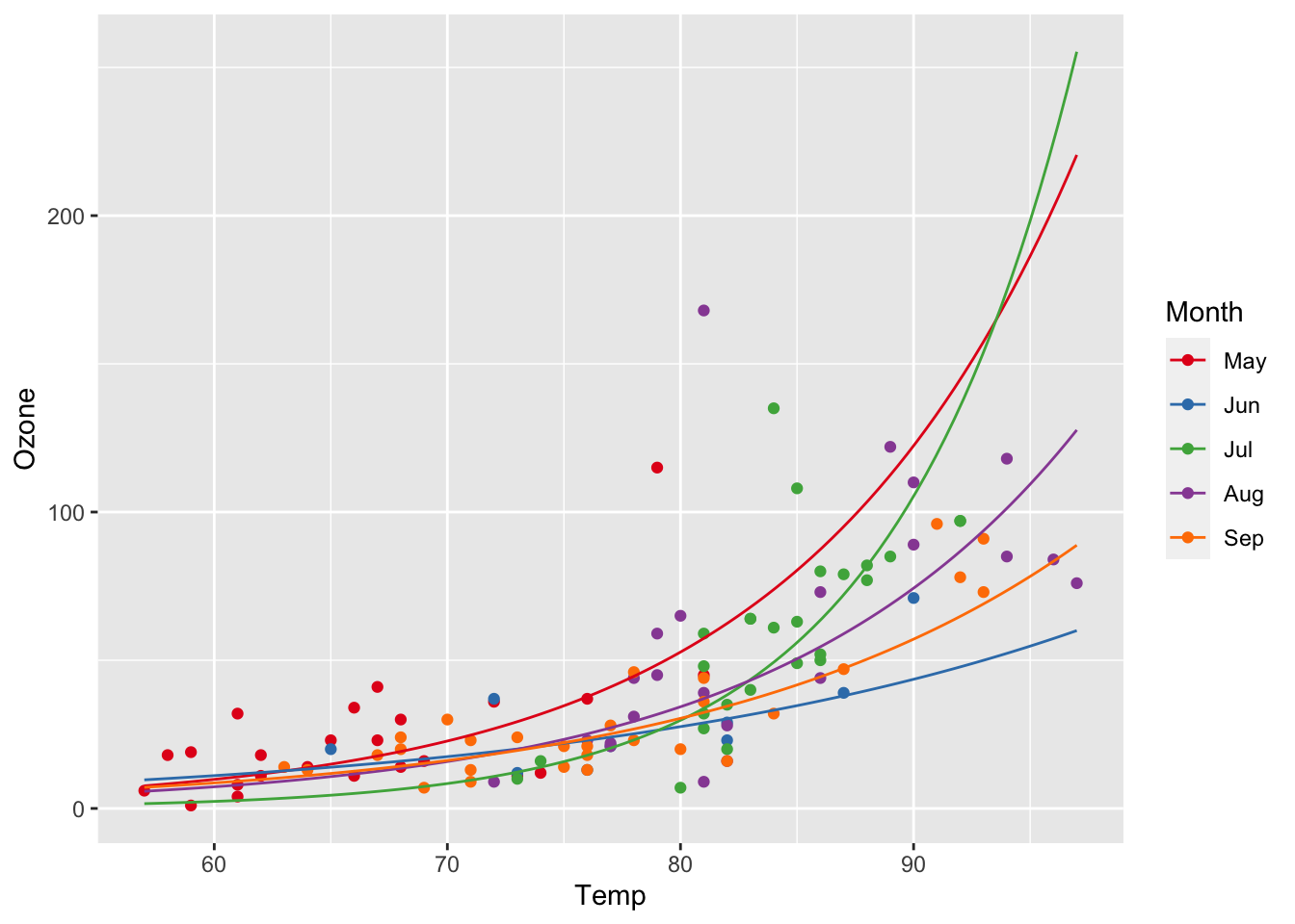

And finally with confidence intervals:

ggplot(airq) +
  geom_point(aes(x = Temp, y = Ozone, col = Month)) +
  geom_ribbon(data = efct, aes(x = Temp, ymin = exp(lower), ymax = exp(upper), fill = Month), alpha = 0.2) +
  geom_line(data = efct, aes(x = Temp, y = exp(fit), col = Month)) +
  scale_color_manual(values = c("#E41A1C", "#377EB8", "#4DAF4A", "#984EA3", "#FF7F00")) +
  scale_fill_manual(values = c("#E41A1C", "#377EB8", "#4DAF4A", "#984EA3", "#FF7F00"))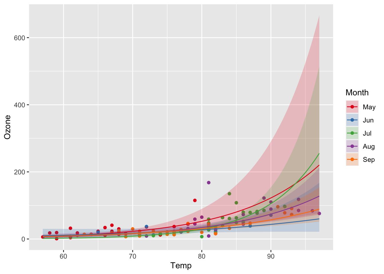

Continuous interactions

We can also specify an interaction between two continuous variables:

lm7 <- lm(logOzone ~ Temp * Wind, data = airq)

summary(lm7)

## 
## Call:
## lm(formula = logOzone ~ Temp * Wind, data = airq)
## 
## Residuals:
##      Min       1Q   Median       3Q      Max 
## -2.31151 -0.28199  0.05219  0.34752  1.12276 
## 
## Coefficients:
##              Estimate Std. Error t value Pr(>|t|)    
## (Intercept) -2.380182   1.306868  -1.821   0.0714 .  
## Temp         0.081641   0.015953   5.118 1.37e-06 ***
## Wind         0.135132   0.115136   1.174   0.2431    
## Temp:Wind   -0.002509   0.001465  -1.713   0.0896 .  
## ---
## Signif. codes:  0 '***' 0.001 '**' 0.01 '*' 0.05 '.' 0.1 ' ' 1
## 
## Residual standard error: 0.5475 on 107 degrees of freedom
## Multiple R-squared:  0.6111, Adjusted R-squared:  0.6002 
## F-statistic: 56.04 on 3 and 107 DF,  p-value: < 2.2e-16

(Intercept): logOzone concentration at 0 windspeed and 0 degrees temperature. If the variables windspeed and temperature are standardised (z-transformed) then the intercept can be interpreted as logOzone concentration at average windspeed and average temperature, which is sometimes more intuitive.

Temp: Increasing temperature by 1 degree F at a windspeed of 0 increases logOzone concentration by 0.08.

Wind: Increasing windspeed by 1 mph is associated with an increase in logOzone concentration of 0.14, when temperature is 0.

Temp:Wind: The effect of temperature on logOzone concentration decreases by -0.003 for every unit increase in windspeed. For example, at zero windspeed, the effect (slope) of temperature on logOzone concentration is 0.082. At a windpeed of 1 mph, the effect decreases to 0.082 - 0.003 = 0.079. Here, the interpretation of the interaction term as windspeed modulating the temperature effect is physically more realistic, while mathematically the interpretation also works the other way round.

Let’s start with the formula showing the additive terms for temperature (\(\beta_1Temp\)) and wind (\(\beta_2Wind\)) and the interaction term between temperature and wind (\(\beta_3TempWind\)):

\[logOzone = \beta_0 +\beta_1Temp +\beta_2Wind +\beta_3Temp*Wind + \epsilon\]

We want to calculate the regression line between temperature and ozone for different levels of windspeed. We can rearrange the equation as follows:

\[y = (\beta_0 +\beta_2Wind) + (\beta_1 +\beta_3Wind) * Temp + \epsilon\]

Now we can say that the intercept is \((\beta_0 + \beta_2Wind)\) and the slope for temperature is \((\beta_1 + \beta_3Wind)\).

We can graph the interaction using the effects package:

efct <- effect("Temp:Wind", mod = lm7, 
               xlevels = list(Temp = seq(57, 97, length.out = 100)))

efct <- as.data.frame(efct)

ggplot(airq) +
  geom_point(aes(x = Temp, y = Ozone, col = Wind)) +
  geom_line(data = efct, aes(x = Temp, y = exp(fit), col = Wind, group = Wind))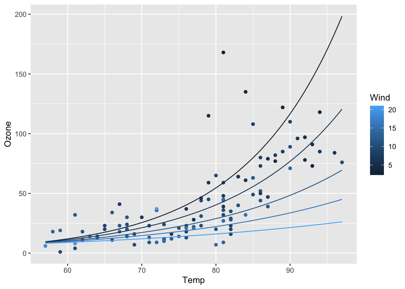

We can also change the values of the modulating variable within the xlevels argument:

efct <- effect("Temp:Wind", mod = lm7, 
               xlevels = list(Temp = seq(57, 97, length.out = 100),
                              Wind = c(0, 10, 20, 30)))

efct <- as.data.frame(efct)

ggplot(airq) +
  geom_point(aes(x = Temp, y = Ozone, col = Wind)) +
  geom_line(data = efct, aes(x = Temp, y = exp(fit), col = Wind, group = Wind))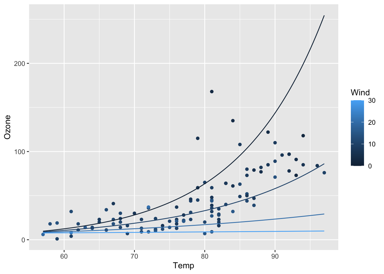

For interpretation, it is often much better to scale the predictors to unit scale (via z-transformation):

airq[, 3:5] <- scale(airq[, 3:5]) # z-transforming Solar, Wind, Temp

lm8 <- lm(logOzone ~ Temp * Wind, data = airq)
summary(lm8)

## 
## Call:
## lm(formula = logOzone ~ Temp * Wind, data = airq)
## 
## Residuals:
##      Min       1Q   Median       3Q      Max 
## -2.31151 -0.28199  0.05219  0.34752  1.12276 
## 
## Coefficients:
##             Estimate Std. Error t value Pr(>|t|)    
## (Intercept)  3.37401    0.05744  58.739  < 2e-16 ***
## Temp         0.54037    0.06017   8.980 1.03e-14 ***
## Wind        -0.21364    0.06017  -3.551 0.000572 ***
## Temp:Wind   -0.08507    0.04967  -1.713 0.089649 .  
## ---
## Signif. codes:  0 '***' 0.001 '**' 0.01 '*' 0.05 '.' 0.1 ' ' 1
## 
## Residual standard error: 0.5475 on 107 degrees of freedom
## Multiple R-squared:  0.6111, Adjusted R-squared:  0.6002 
## F-statistic: 56.04 on 3 and 107 DF,  p-value: < 2.2e-16

Given the interpretation above, the coefficient for Temp now indicates the increase in logOzone with an increase in temperature by 1 standard deviation (9.5 F) at mean windspeed (9.9 mph).

Again plotting the regression model:

efct <- effect("Temp:Wind", mod = lm8, 
               xlevels = list(Temp = seq(-2, 2, length.out = 100)))

efct <- as.data.frame(efct)

ggplot(airq) +
  geom_point(aes(x = Temp, y = Ozone, col = Wind)) +
  geom_line(data = efct, aes(x = Temp, y = exp(fit), col = Wind, group = Wind))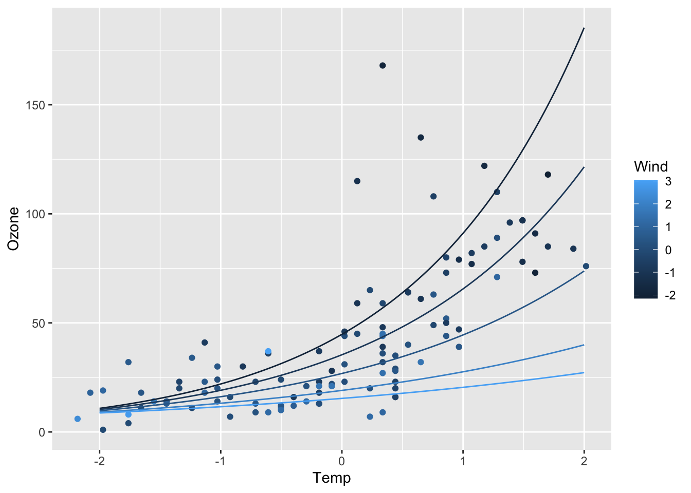

Model selection

AIC

The Akaike Information Criterion (AIC) balances the goodness of fit with a penalty for model complexity. AIC is defined such that the smaller the value of AIC the better the model. Compare models based on the Akaike Information Criterion:

AIC(lm1, lm2, lm3)

##     df      AIC
## lm1  5 170.8251
## lm2  6 168.5865
## lm3  7 168.0743

What is the advantage of AIC over \(R^2\)?

c(summary(lm1)$r.squared, summary(lm2)$r.squared, summary(lm3)$r.squared)

## [1] 0.6644239 0.6769963 0.6842246

c(summary(lm1)$adj.r.squared, summary(lm2)$adj.r.squared, summary(lm3)$adj.r.squared)

## [1] 0.6550153 0.6648075 0.6691876

Stepwise elimination

R has several functions for performing model searches, e.g. based on the Akaike Information Criterion. Such functions make the process of model selection efficient, particularly when there are lots of predictor variables. In the seminar, we looked at manual backward and forward model selection:

Backward elimination:

Start with a full model including potential transformations and polynomials
Work your way backwards by eliminating non-significant variables
Compare models using AIC and \(R_{adj}\)

Forward elimination:

Start with a single predictor
Add variables and assess their significance
Compare models using AIC and \(R_{adj}\)

One advantage of doing model reductions by hand is that you can impose some logical structure on the process, based on your understanding of the data and the underlying processes.

Exaustive search

Here, we want to show you an alternative approach to backward/forward model selection: exhaustive model comparison. Exhaustive model comparison makes use of the power of modern computers to compare all possible model combinations. For doing so, we use the function dredge() in the package MuMIn:

options(na.action = "na.fail")  # Prevent fitting models when data set changes due to NAs

fit_full <- lm(logOzone ~ (Temp * Wind + Solar) * Month, data = airq)

fit_all <- MuMIn::dredge(global.model = fit_full, rank = AIC)

The result is a list of competing models:

head(fit_all, n = 5)

## Global model call: lm(formula = logOzone ~ (Temp * Wind + Solar) * Month, data = airq)
## ---
## Model selection table 
##     (Int) Mnt    Slr    Tmp     Wnd Mnt:Tmp Mnt:Wnd  Tmp:Wnd Mnt:Tmp:Wnd df  logLik   AIC delta
## 143 3.367     0.2365 0.4681 -0.2197                 -0.09930              6 -77.967 167.9  0.00
## 496 3.717   + 0.2307 0.7637 -0.5348       +       + -0.36290           + 22 -63.100 170.2  2.27
## 15  3.416     0.2293 0.4686 -0.2190                                       5 -80.413 170.8  2.89
## 80  3.482   + 0.1954 0.4944 -0.1406               +                      13 -73.074 172.1  4.21
## 208 3.469   + 0.2002 0.4919 -0.2188               + -0.06214             14 -72.498 173.0  5.06
##     weight
## 143  0.569
## 496  0.183
## 15   0.134
## 80   0.069
## 208  0.045
## Models ranked by AIC(x)

The first model in this list is the best according to AIC and then remaining models are ranked from next best to worst by difference in AIC, \(\Delta AIC\), with respect to the best model. Some of these lower-rank models are quite similar to each other in terms of AIC, i.e. model 2 and model 3 in this list, and model 4 and model 5.

We can extract the best model according to AIC like this:

model_selection <- get.models(fit_all, delta < 2) # Returns a list of models, in our case only one!
model <- model_selection[[1]]
model

## 
## Call:
## lm(formula = logOzone ~ Solar + Temp + Wind + Temp:Wind + 1, 
##     data = airq)
## 
## Coefficients:
## (Intercept)        Solar         Temp         Wind    Temp:Wind  
##      3.3670       0.2365       0.4681      -0.2197      -0.0993

6. Multiple regression and model selection

Humboldt-Universität zu Berlin | Geography Department

Content

Packages

Data

Exploratory analysis

Multiple regression formula

Dummy variables

Variable intercept

Example

Interaction terms

Estimate interaction effects

Example

The `effects` package

Continuous interactions

Model selection

AIC

Stepwise elimination

Exaustive search

6. Multiple regression and model selection

Humboldt-Universität zu Berlin | Geography Department

Content

Packages

Data

Exploratory analysis

Multiple regression formula

Dummy variables

Variable intercept

Example

Interaction terms

Estimate interaction effects

Example

The effects package

Continuous interactions

Model selection

AIC

Stepwise elimination

Exaustive search

The `effects` package