- Packages
- Data
- Model types
- Classification error
- Cross-Validation
- K-Fold Cross-validation
- Leave-one-out cross-validation
- Linear Discriminant Analysis
- Model fitting
- Examine model
- Model output
- Confusion matrix (training error)
- Confusion matrix (test error)
- Quantitative predictions
- Cross-validation (self-made)
- Cross-validation (Caret)
- References
LDA and Model assessment in R
Humboldt-Universität zu Berlin | Geography Department
Packages
library(MASS)    # includes linear discriminant function analysis
library(caret)   # cross-validation
library(ggplot2) # graphics
Data
For this exercise, we use the taxon data from the R Book
(Crawley, 2012).
taxa <- read.table("data/taxonomy.txt", header=T, stringsAsFactors = T)
head(taxa)
## Taxon Petals Internode Sepal Bract Petiole Leaf Fruit
## 1 I 5.621498 29.48060 2.462107 18.20341 11.27910 1.128033 7.876151
## 2 I 4.994617 28.36025 2.429321 17.65205 11.04084 1.197617 7.025416
## 3 I 4.767505 27.25432 2.570497 19.40838 10.49072 1.003808 7.817479
## 4 I 6.299446 25.92424 2.066051 18.37915 11.80182 1.614052 7.672492
## 5 I 6.489375 25.21131 2.901583 17.31305 10.12159 1.813333 7.758443
## 6 I 5.785868 25.52433 2.655643 17.07216 10.55816 1.955524 7.880880The dataset contains seven morphological variables
(Petals, Internode, Sepal,
Bract, Petiole, Leaf,
Fruit) that might be useful for separating the categorical
response variable Taxon. The Taxon variable is
a factor variable with four factor levels: I,
II, III, IV. The
table() function reveals that there are 30
individuals/observations per factor level.
table(taxa$Taxon)##
## I II III IV
## 30 30 30 30Model types
Discriminative models
- Estimate conditional models Pr[Y|X]
- Logistic regression
Generative models
- Estimate joint probability Pr[Y,X]=Pr[Y|X]⋅Pr[X]
- Estimates not only probability of labels but also the features
- Once model is fit, can be used to generate data
- LDA, QDA, Naive Bayes
Generative models can be used to generate data (Pr[X]) and they often offer more insights into the data (interpretation). On the downside, these models sometimes work worse, particularly when assumptions are violated.
Classification error
The prediction (or generalization) error estimates how well our model predicts unobserved data, i.e., data that was not used involved in the training of the model. The term classification error relates to models that predict discrete classes as opposed to continuous variables. It is common to asses the accuracy of categorical predictions by constructing a confusion matrix. From the confusion matrix, we can estimate several types of errors.
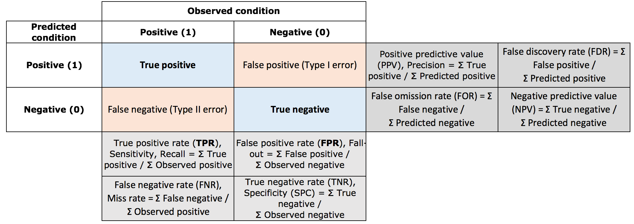
Overall accuracy = ∑true positives+∑true negatives∑total samples
Omission error (of positives) = FNR; Commission error (of positives) = FDR.
These errors also have analog terminology used in hypothesis testing. The type I error (the incorrect rejection of a true null hypothesis) describes the detection an effect that is not present). The type II error (failure to reject a false null hypothesis) is the failure to detect an effect that is present.
Cross-Validation
Sometimes, there are not enough data to split into training and test sample. Probably the simplest and most widely used method for estimating prediction error is cross-validation.
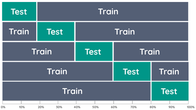
K-Fold Cross-validation
K-fold cross-validation uses part of the available data to fit the model, and a different part to test it. We split the data into K roughly equal-sized parts. Typical choices of K are between 5 and 10. When K = 5, the scenario looks like this:
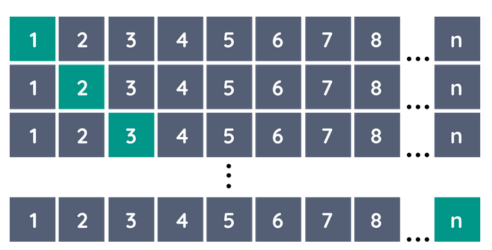
Leave-one-out cross-validation
The case K = N is known as leave-one-out cross-validation. In this case, for the i’th observation the fit is computed using all the data except the i’th.
Linear Discriminant Analysis
Model fitting
The MASS package provides functions to conduct
discriminant function analysis. We will use lda() to carry
out a linear discriminant analysis on the taxa dataset. By now, you are familiar
with the formula style: response ~ explanatory variables.
The . denotes all variables in the taxa dataset except the
variable specified as response.
lda_model <- MASS::lda(Taxon ~ ., data=taxa)The lda object (in this example lda_model)
contains the following components (and more):
prior: the prior probabilities used.
means: the group means.
scaling: a matrix of coefficients that transforms observations to discriminant functions.
svd: the singular values, which give the ratio of the between- and within-group standard deviations on the linear discriminant variables.
N: The number of observations used.
counts: The number of observations per class.
Examine model
By default, equal prior probabilities are prescribed to each class:
lda_model$prior## I II III IV
## 0.25 0.25 0.25 0.25lda_model$svd## [1] 20.589120 9.098563 8.750050The singular values are analogous to the eigenvalues of the Principal Component Analysis, except that LDA does not maximize the variance of a component, instead it maximizes the separability (defined by the between and within-group standard deviation). Thus, the “proportion of trace” is the proportion of between-class variance that is explained by successive discriminant functions.
lda_model$svd^2 / sum(lda_model$svd^2)## [1] 0.7267985 0.1419332 0.1312682Hence, 72.7% of the between-class variance is explained by the first linear discriminant function (LD1).
As always, you get a printed overview of all essential model results by printing the model object:
lda_model## Call:
## lda(Taxon ~ ., data = taxa)
##
## Prior probabilities of groups:
##    I   II  III   IV
## 0.25 0.25 0.25 0.25
##
## Group means:
## Petals Internode Sepal Bract Petiole Leaf Fruit
## I 5.476128 27.91886 2.537955 18.60268 10.864184 1.508029 7.574642
## II 7.035078 27.69834 2.490336 18.47557 8.541085 1.450260 7.418702
## III 6.849666 27.99308 2.446003 18.26330 9.866983 2.588555 7.482349
## IV 6.768464 27.78503 4.532560 18.42953 10.128838 1.645945 7.467917
##
## Coefficients of linear discriminants:
## LD1 LD2 LD3
## Petals -0.01891137 -0.034749952 -0.559080267
## Internode 0.03374178 -0.009670875 -0.008808043
## Sepal 3.45605170 0.500418135 -0.401274694
## Bract 0.07557480 -0.068774714 0.024930728
## Petiole 0.25041949 0.343892260 1.249519047
## Leaf -1.13036429 3.008335468 -0.647932763
## Fruit 0.18285691 0.208370808 0.269924935
##
## Proportion of trace:
## LD1 LD2 LD3
## 0.7268 0.1419 0.1313The number of discriminant functions that can be extracted depends on
the number of groups and the number of variables – it is the lesser of
the degrees of freedom for groups (number of groups minus one) and the
number of variables (Tabachnick & Fidell 1996). The scaling
coefficients show, LD1 is largely explained by the variable
Sepal. Plotting Sepal versus Leaf length confirms this:
plot(taxa$Sepal, taxa$Leaf, col=taxa$Taxon, type="n")
text(taxa$Sepal, taxa$Leaf, labels=as.character(taxa$Taxon), col=as.numeric(taxa$Taxon))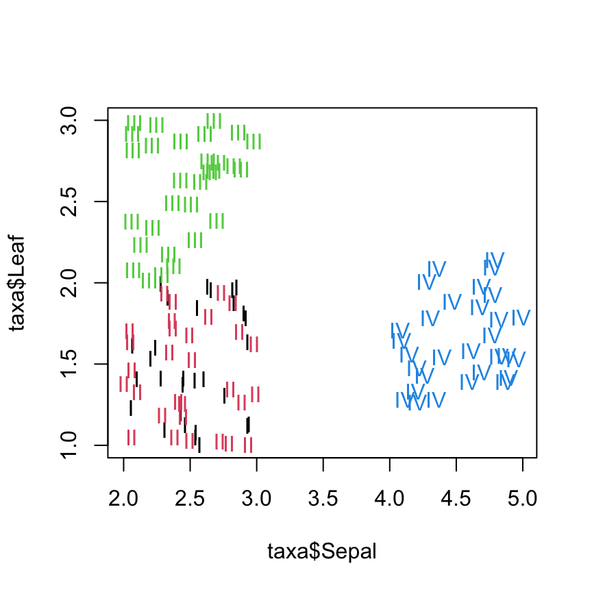
Model output
Applying the predict() function to the LDA model yields
the following results (see ?predict.lda):
lda_model$class: The predicted class based on the
maximum posterior probability (MAP)
lda_model$posterior: posterior probabilities for the
classes
lda_model$x: the scores of test cases for all
discriminant functions
lda_prediction <- predict(lda_model)
str(lda_prediction)
## List of 3
## $ class : Factor w/ 4 levels "I","II","III",..: 1 1 1 1 1 1 1 1 1 1 ...
## $ posterior: num [1:120, 1:4] 1 1 1 0.999 0.883 ...
## ..- attr(*, "dimnames")=List of 2
## .. ..$ : chr [1:120] "1" "2" "3" "4" ...
## .. ..$ : chr [1:4] "I" "II" "III" "IV"
## $ x : num [1:120, 1:3] -0.624 -1.099 -0.285 -2.568 -0.419 ...
## ..- attr(*, "dimnames")=List of 2
## .. ..$ : chr [1:120] "1" "2" "3" "4" ...
## .. ..$ : chr [1:3] "LD1" "LD2" "LD3"We can glue together the posterior-probabilities and the predicted
class vector (with cbind() to show for each row, the
predicted class represents the class with the maximum posterior
probability
i <- sample(120) # random row
head(cbind(round(lda_prediction$posterior[i,], 4), class=lda_prediction$class[i]))
## I II III IV class
## 49 0.1831 0.7612 0.0557 0 2
## 101 0.0000 0.0000 0.0000 1 4
## 65 0.0005 0.0051 0.9944 0 3
## 25 0.9892 0.0108 0.0000 0 1
## 74 0.0188 0.1651 0.8161 0 3
## 100 0.0000 0.0000 0.0000 1 4The LDA scores (the transformed values in LDA space) for all
observations can be accessed via $x:
head(lda_prediction$x)## LD1 LD2 LD3
## 1 -0.6240211 -1.6810963 3.0303236
## 2 -1.0988293 -1.6768377 2.8176493
## 3 -0.2850537 -2.3155720 2.5934923
## 4 -2.5680633 -0.2811099 3.1292050
## 5 -0.4189485 0.2502168 0.4620391
## 6 -1.2922825 0.7685348 1.4317043A nice way of displaying the results of a linear discriminant analysis (LDA) is to plot the LDA scores as histograms or scatterplots. A stacked histogram shows the scores of the discriminant functions separately for each group.
ldahist(data = lda_prediction$x[,], g=taxa$Taxon)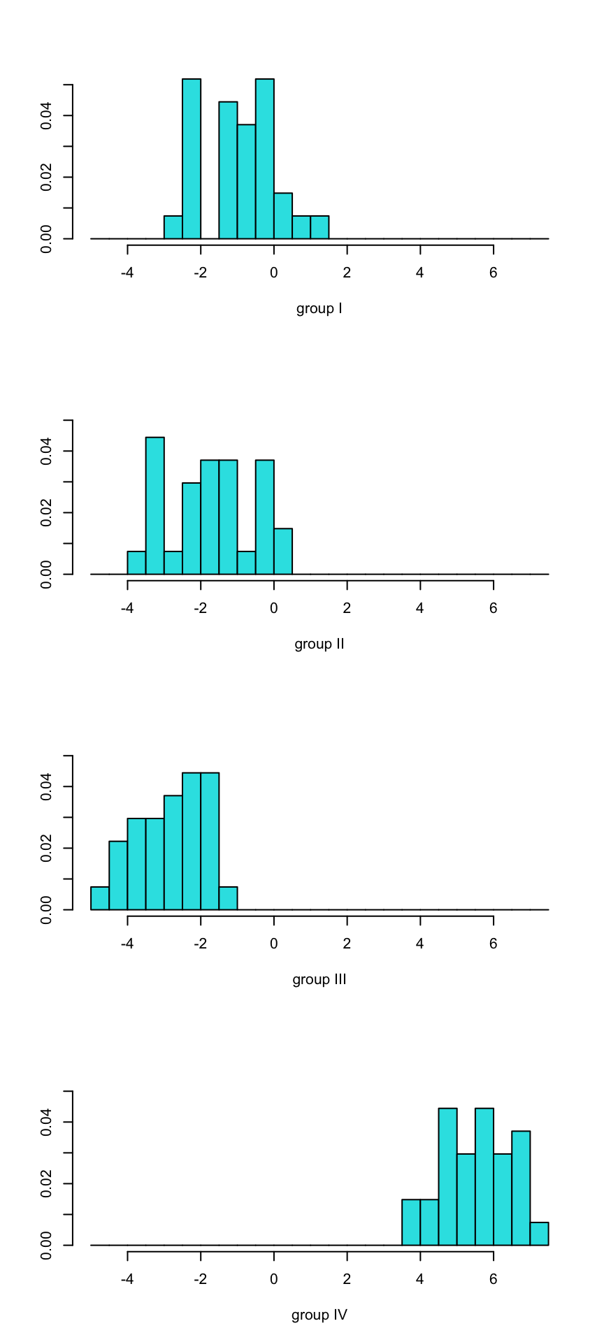
We can also produce a scatterplot showing how the groups separate
along the LDA axes (below). LD1 separates taxum IV from the
other taxa. LD2 separates well III from I and
II. LD3 seems to separate taxum I from the
other groups.
plot(lda_model, col=as.numeric(taxa$Taxon)) # assign color code based on factor code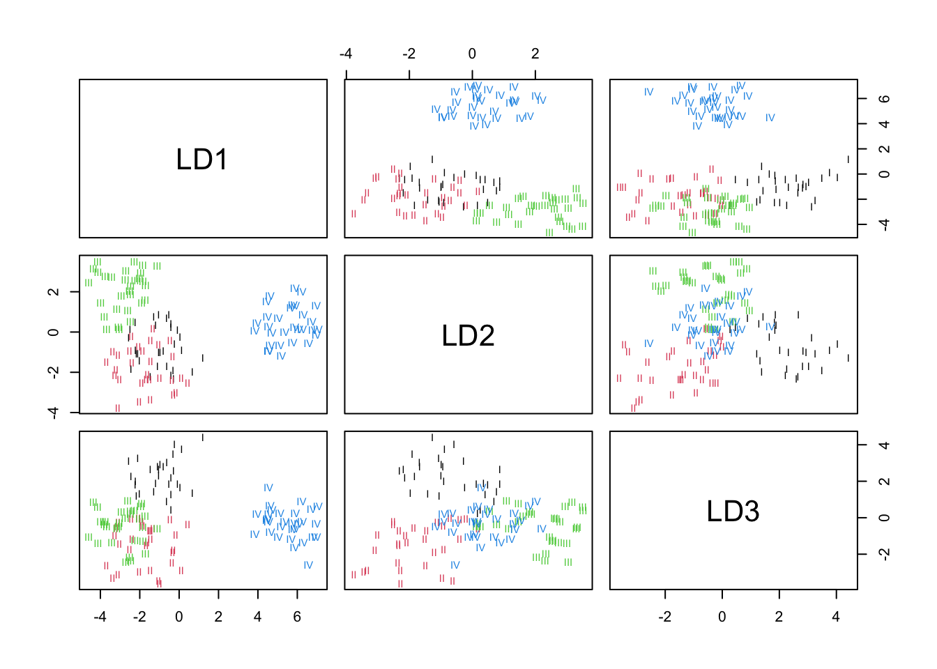
Confusion matrix (training error)
To check how well the model predicts our training data, we can
construct a confusion matrix of the fitted vs observed Taxa using the
table function.
conf <- table(list(predicted=lda_prediction$class, observed=taxa$Taxon))
conf
## observed
## predicted I II III IV
## I 29 0 0 0
## II 0 30 0 0
## III 1 0 30 0
## IV 0 0 0 30We can calculate the categorical accuracy measures using simple matrix arithmetic…
# Precision (Positive predicted value)
diag(conf) / rowSums(conf)## I II III IV
## 1.0000000 1.0000000 0.9677419 1.0000000# Sensitivity
diag(conf) / colSums(conf)## I II III IV
## 0.9666667 1.0000000 1.0000000 1.0000000Alternatively, the caret package includes functionality that makes this easier:
confusionMatrix(conf)## Confusion Matrix and Statistics
##
##          observed
## predicted  I II III IV
##       I   29  0   0  0
##       II   0 30   0  0
##       III  1  0  30  0
##       IV   0  0   0 30
##
## Overall Statistics
##
## Accuracy : 0.9917
## 95% CI : (0.9544, 0.9998)
## No Information Rate : 0.25
## P-Value [Acc > NIR] : < 2.2e-16
##
## Kappa : 0.9889
##
## Mcnemar's Test P-Value : NA
##
## Statistics by Class:
##
## Class: I Class: II Class: III Class: IV
## Sensitivity 0.9667 1.00 1.0000 1.00
## Specificity 1.0000 1.00 0.9889 1.00
## Pos Pred Value 1.0000 1.00 0.9677 1.00
## Neg Pred Value 0.9890 1.00 1.0000 1.00
## Prevalence 0.2500 0.25 0.2500 0.25
## Detection Rate 0.2417 0.25 0.2500 0.25
## Detection Prevalence 0.2417 0.25 0.2583 0.25
## Balanced Accuracy 0.9833 1.00 0.9944 1.00Confusion matrix (test error)
The previous error estimates show the training error.
The lda() function also includes an easy way to estimate
the test error using leave-one-out cross-validation by
specifying CV=T.
lda_model2 <- lda(Taxon ~ ., data=taxa, CV=T)
conf2 <- table(list(predicted=lda_model2$class, observed=taxa$Taxon))
caret::confusionMatrix(conf2)
## Confusion Matrix and Statistics
##
## observed
## predicted I II III IV
## I 29 1 0 0
## II 0 28 0 0
## III 1 1 30 0
## IV 0 0 0 30
##
## Overall Statistics
##
## Accuracy : 0.975
## 95% CI : (0.9287, 0.9948)
## No Information Rate : 0.25
## P-Value [Acc > NIR] : < 2.2e-16
##
## Kappa : 0.9667
##
## Mcnemar's Test P-Value : NA
##
## Statistics by Class:
##
## Class: I Class: II Class: III Class: IV
## Sensitivity 0.9667 0.9333 1.0000 1.00
## Specificity 0.9889 1.0000 0.9778 1.00
## Pos Pred Value 0.9667 1.0000 0.9375 1.00
## Neg Pred Value 0.9889 0.9783 1.0000 1.00
## Prevalence 0.2500 0.2500 0.2500 0.25
## Detection Rate 0.2417 0.2333 0.2500 0.25
## Detection Prevalence 0.2500 0.2333 0.2667 0.25
## Balanced Accuracy 0.9778 0.9667 0.9889 1.00Quantitative predictions
For quantitative predictions from regression, we also compare the observed vs the predicted values. Usually, we calculate some kind of average difference:
Mean Squared Error (MSE)
MSE=1n∑ni=1(yi−^yi)2=1nSSE
Root Mean Squared Error (RMSE)
RMSE=√(MSE)
Mean Absolute Error (MAE)
1n∑ni=1|yi−^yi|
Cross-validation (self-made)
Recall the airquality dataset that we used in previous sessions. Our goal is now to assess, how well the following linear model predicts ozone concentrations based on air temperature and solar radiation. We will write a loop to conduct a K-Fold cross-validation.
fit <- lm(log(Ozone) ~ I(Temp^2) + Solar.R, data = airquality)
summary(fit)
##
## Call:
## lm(formula = log(Ozone) ~ I(Temp^2) + Solar.R, data = airquality)
##
## Residuals:
## Min 1Q Median 3Q Max
## -1.9178 -0.3366 0.0389 0.3031 1.4087
##
## Coefficients:
## Estimate Std. Error t value Pr(>|t|)
## (Intercept) 5.150e-01 2.247e-01 2.292 0.0238 *
## I(Temp^2) 3.972e-04 3.644e-05 10.902 < 2e-16 ***
## Solar.R 2.496e-03 5.860e-04 4.259 4.41e-05 ***
## ---
## Signif. codes: 0 '***' 0.001 '**' 0.01 '*' 0.05 '.' 0.1 ' ' 1
##
## Residual standard error: 0.5366 on 108 degrees of freedom
## (42 observations deleted due to missingness)
## Multiple R-squared: 0.6229, Adjusted R-squared: 0.616
## F-statistic: 89.22 on 2 and 108 DF, p-value: < 2.2e-16First, we use the caret package to slice the dataset
into 10 folds (sub-samples):
# remove NA's
airquality_no_na <- na.omit(airquality)

folds <- createFolds(airquality_no_na$Ozone, k = 10)
You’ll notice that we provide createFolds() only with a
vector and not the entire dataset. The key here is, the function returns
a list of row indices instead of the actual data.
class(folds)## [1] "list"folds[1:4]## $Fold01
## [1] 10 18 55 68 71 73 76 83 101 107 111
##
## $Fold02
## [1] 13 28 34 42 45 46 86 90 91 93 100 109
##
## $Fold03
## [1] 8 11 24 54 58 62 70 79 82 89
##
## $Fold04
## [1] 2 5 12 30 31 49 53 60 77 106 110We can write a function that takes two attributes as input: 1) the
entire data.frame (data) and 2) the indices of a fold
(i). We call our function crossValidateLM.
crossValidateLM <- function(data, i){

  # all rows that are not in the fold are copied into a training dataset
  train <- data[-i, ]

  # all rows that are in the fold are used as test dataset
  test <- data[i, ]

  # fit a model using the training dataset
  fit <- lm(log(Ozone) ~ I(Temp^2) + Solar.R, data = train)

  # apply the model to the test dataset
  pred_log <- predict(fit, newdata = test)

  # back-transform log Ozone to Ozone
  pred <- exp(pred_log)

  # extract the observed Ozone concentration (reference)
  ref <- test$Ozone

  # return a data.frame with two columns containing the cross-validated
  # predictions for the fold and the corrsponding reference observations
  return(data.frame(Prediction = pred,
                    Reference = ref))
}
Let’s test our function on the first fold:
cv_first_fold <- crossValidateLM(airquality_no_na, folds[[1]])

head(cv_first_fold)
## Prediction Reference
## 14 21.74296 14
## 22 32.58521 11
## 88 36.00532 52
## 106 30.56817 65
## 110 21.28769 23
## 112 29.80983 44ggplot(cv_first_fold, aes(x = Reference, y = Prediction)) +
geom_point() +
xlim(0, 175) +
ylim(0, 175) +
geom_abline(intercept = 0, slope = 1)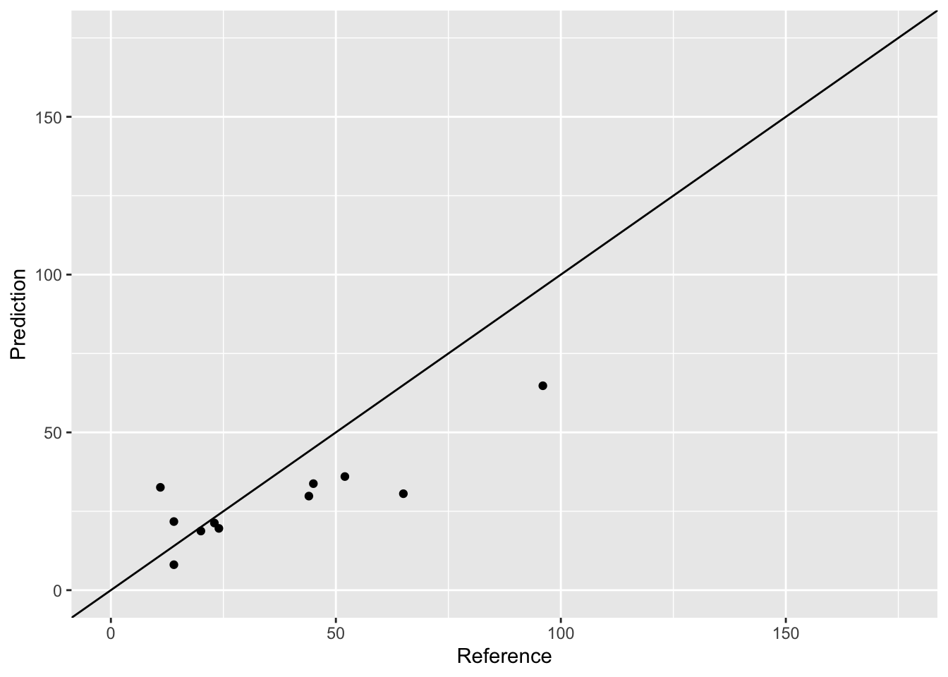
Looks good but we also need the predictions from the other folds. We can all gather them together by writing a loop from fold 1 to fold 10:
# create empty data.frame
cv_all_folds <- data.frame(Prediction = numeric(0), Reference = numeric(0))

for(i in folds){
  # add the rows of the fold
  cv_all_folds <- rbind(cv_all_folds, crossValidateLM(airquality_no_na, i))
}

ggplot(cv_all_folds, aes(x = Reference, y = Prediction)) +
  geom_point() +
  xlim(0, 175) +
  ylim(0, 175) +
  geom_abline(intercept = 0, slope = 1)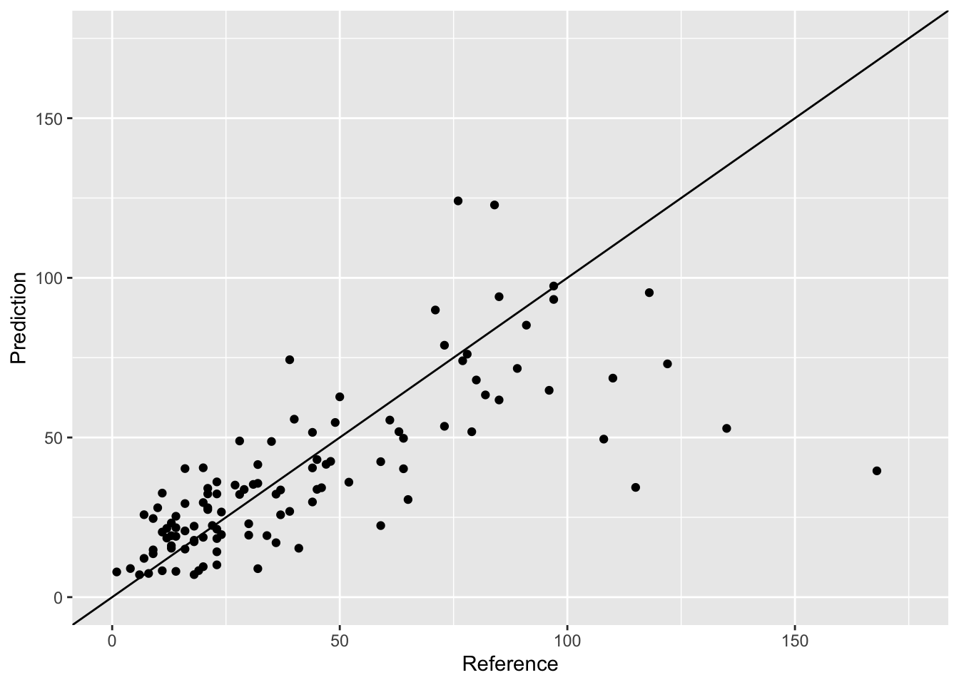
Now, as we have our cross-validated predictions and reference observations in one data.frame, we can calculate the root-mean-squared error (RMSE), mean squared error (MSE), and mean absolute error (MAE).
mse <- function(x, y){mean((x - y)^2)}
mse(x = cv_all_folds$Prediction, y = cv_all_folds$Reference)
## [1] 538.0367rmse <- function(x, y){sqrt(mean((x - y)^2))}
rmse(x = cv_all_folds$Prediction, y = cv_all_folds$Reference)## [1] 23.19562mea <- function(x, y){mean(abs(x - y))}
mea(x = cv_all_folds$Prediction, y = cv_all_folds$Reference)## [1] 14.65878Cross-validation (Caret)
You probably realize, writing you own cross-validation function is
not hard once you understand functions and loops in R. The caret
package (and numerous other packages) provide you with
cross-validation functions for which you don’t have to write that many
lines of code. This is convenient, as long as those functions work with
the models that you are interested in. Here is an example using a linear
regression model.
# define training control
train.control <-  trainControl(method="LOOCV")

# train mean height model
loocv <- train(log(Ozone) ~ I(Temp^2) + Solar.R, data = airquality_no_na, method = "lm", trControl = train.control)
loocv
## Linear Regression
##
## 111 samples
## 2 predictor
##
## No pre-processing
## Resampling: Leave-One-Out Cross-Validation
## Summary of sample sizes: 110, 110, 110, 110, 110, 110, ...
## Resampling results:
##
## RMSE Rsquared MAE
## 0.5461937 0.5987285 0.4187436
##
## Tuning parameter 'intercept' was held constant at a value of TRUEA note about how R2 is calculated by caret: it takes the approach of computing the correlation between the observed and predicted values and squaring the value. So, it is NOT the coefficient of determination of the model. Especially when the model is poor, this can lead to differences between this estimator and the more widely known estimate derived form linear regression models.
# define training control
lmd <-  lm(log(Ozone) ~ I(Temp^2) + Solar.R, data = airquality_no_na)

# R2 estimated from OLS
summary(lmd)[["r.squared"]]
## [1] 0.6229448# adjusted R2 estimated from OLS
summary(lmd)[["adj.r.squared"]]## [1] 0.6159623# R2 from caret
loocv$results$Rsquared## [1] 0.5987285Also, the RMSE is on the log-scale since the model predicts log(Ozone). We cannot simply square the RMSE for back-transformation. You need to calculate the RMSE on the back-transformed predictions yourself. See below, how to access the predictions.
pred <- loocv$pred
head(pred)
## pred obs rowIndex intercept
## 1 2.751203 3.713572 1 TRUE
## 2 2.857273 3.583519 2 TRUE
## 3 3.068884 2.484907 3 TRUE
## 4 2.818412 2.890372 4 TRUE
## 7 2.929038 3.135494 5 TRUE
## 8 2.110938 2.944439 6 TRUEggplot(pred, aes(x = exp(obs), y = exp(pred))) +
geom_point() +
geom_abline(intercept = 0, slope = 1)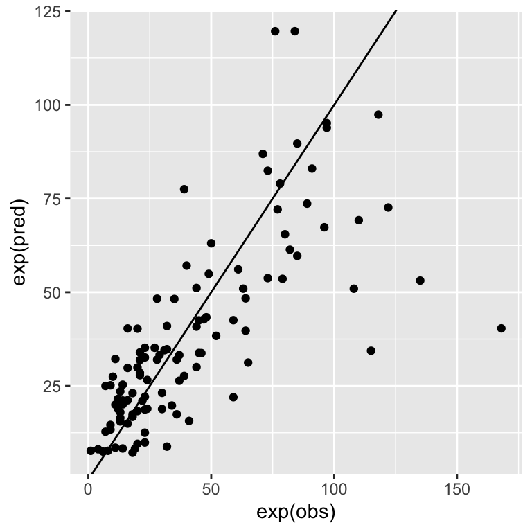
References
Crawley, MJ (2012). The R Book. 2nd edition. John Wiley & Sons.]
Copyright © 2024 Humboldt-Universität zu Berlin. Department of Geography.
![]()