Content
- Hypothesis testing
- t-test
- F-test
- p-value
- Analysis of variance (ANOVA) in R
- Tukey’s multiple comparison test
library(ggplot2) # load ggplot2 package for visualization
library(tidyr) # data wrangling package: change from wide to long format
library(dplyr) # data manipulation: mutateWe will use the soil data set from Crawley (2012). The data come from an experiment in which crop yields per unit area were measured from 10 randomly selected fields on each of three soil types. All fields were sown with the same variety of seed and provided with the same fertilizer and pest control inputs. The underlying question is whether soil type significantly affects crop yield.
yields <- read.table("data/yields.txt", sep = ";", header = TRUE)
head(yields)
## plotid sand clay loam
## 1 1 6 17 13
## 2 2 10 15 16
## 3 3 8 3 9
## 4 4 6 11 12
## 5 5 14 14 15
## 6 6 17 12 16summary(yields)## plotid sand clay loam
## Min. : 1.00 Min. : 6.00 Min. : 3.00 Min. : 9.0
## 1st Qu.: 3.25 1st Qu.: 7.25 1st Qu.:10.25 1st Qu.:13.0
## Median : 5.50 Median : 9.50 Median :12.00 Median :14.5
## Mean : 5.50 Mean : 9.90 Mean :11.50 Mean :14.3
## 3rd Qu.: 7.75 3rd Qu.:11.00 3rd Qu.:13.75 3rd Qu.:16.0
## Max. :10.00 Max. :17.00 Max. :17.00 Max. :18.0Reshape and summarize:
yields_tidy <- yields %>% pivot_longer(cols = -plotid,
                                       names_to = "soiltype",
                                       values_to = "yield")
head(yields_tidy)
## # A tibble: 6 × 3
## plotid soiltype yield
## <int> <chr> <int>
## 1 1 sand 6
## 2 1 clay 17
## 3 1 loam 13
## 4 2 sand 10
## 5 2 clay 15
## 6 2 loam 16yields_tidy_summary <- yields_tidy %>%
group_by(soiltype) %>%
summarize(mean = mean(yield))
yields_tidy_summary## # A tibble: 3 × 2
## soiltype mean
## <chr> <dbl>
## 1 clay 11.5
## 2 loam 14.3
## 3 sand 9.9Visualize:
ggplot(yields_tidy, aes(x = soiltype, y = yield)) +
  geom_boxplot() +
  geom_hline(yintercept = mean(yields_tidy$yield), linetype = "dashed") +
  geom_point(data = yields_tidy_summary, aes(x = soiltype, y = mean), shape = 2)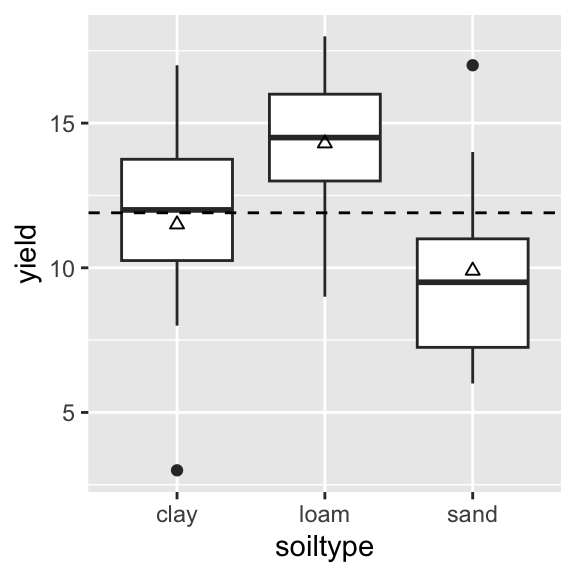
Is the difference in yields between soil types meaningful?
We might ask the following question: Are the yields the same on loam and sand? To test this, we formulate a precise Null hypothesis H0: The average yields are equal on both soil types, that is μloam=μsand; and a congruent alternative hypothesis HA: The average yields are not equal on both soil types, that is μloam≠μsand.
The principal idea behind hypothesis testing is to formulate the problem - here the difference in means - in form of a test statistic and calculate how probable it would be to get such a value of the test statistic or a more extreme one by chance in repeat data sampling assuming that H0 is true. This probability is the p-value. If the p-value is very small, we might safely reject H0 and call the difference in means in this case significant.
Even though the p-value has a clear definition, it is very often misinterpreted. Here are the common pitfalls:
If you’re interested in the abuse of p-values, you can keep reading here.
The hypothesis test for two means is called a t-test (or Student’s t-test). The basic idea behind the t-test is that the difference between two means would be exact zero if they were the same. Hence, under the assumption of H0, a large difference is very unlikely.
Lets calculate the t-value, degrees of freedom, and p-value for our example:
t.test(x = yields$loam, y = yields$sand, alternative = "two.sided", var.equal = TRUE)##
## Two Sample t-test
##
## data: yields$loam and yields$sand
## t = 3.1375, df = 18, p-value = 0.005692
## alternative hypothesis: true difference in means is not equal to 0
## 95 percent confidence interval:
## 1.453711 7.346289
## sample estimates:
## mean of x mean of y
## 14.3 9.9The difference in sample means observed for our samples is very unlikely under the assumption of H0 being true. We thus might safely reject H0 and conclude that the mean yields are significantly different between both soil types.
The F-test aims at testing the difference in the variances between two samples.
The Null hypothesis H0
is:
The variances are equal σ2loam=σ2sand.
The alternative hypothesis H1
is:
The variances are not equal σ2loam≠σ2sand.
The test statistic is the F-statistic, calculated as the ratio of the sample variances:
Fs=s22s21.
Assuming that H0 is true, the F-statistic follows the F-distribution with two parameters:
v1=n1−1 and v2=n2−1.
The F-test can be easily calculated in R:
var.test(x = yields$loam, y = yields$sand, alternative = "two.sided")##
## F test to compare two variances
##
## data: yields$loam and yields$sand
## F = 0.56776, num df = 9, denom df = 9, p-value = 0.4119
## alternative hypothesis: true ratio of variances is not equal to 1
## 95 percent confidence interval:
## 0.1410233 2.2857947
## sample estimates:
## ratio of variances
## 0.5677591The probability of getting an F-statistic as extreme as the one observed is very likely under the assumption of H0 being true. Hence, we cannot reject H0 and thus cannot say that there are significant differences in variance between both soil types.
The t-test assumes that the samples are normally distributed. The t-test moreover assumes equal variances for both samples, an assumption you can relax using the Welch t-Test:
t.test(x = yields$loam, y = yields$sand, alternative = "two.sided", var.equal = FALSE)##
## Welch Two Sample t-test
##
## data: yields$loam and yields$sand
## t = 3.1375, df = 16.728, p-value = 0.006094
## alternative hypothesis: true difference in means is not equal to 0
## 95 percent confidence interval:
## 1.437576 7.362424
## sample estimates:
## mean of x mean of y
## 14.3 9.9ANOVA assumes variance homogeneity between groups. We can use a simple F-test to check if the variances of two groups are equal (homogeneous). Alternatively, Bartlett’s test can be applied to compare variances of more than two samples. In the example below, we test if the variances of all three soil types are equal (H0: variance is homogeneous):
# argument x takes the numeric yield vector as input
# argument g takes the factor vector of the soil types as input
bartlett.test(x = yields_tidy$yield, g = yields_tidy$soiltype)
##
## Bartlett test of homogeneity of variances
##
## data: yields_tidy$yield and yields_tidy$soiltype
## Bartlett's K-squared = 1.2764, df = 2, p-value = 0.5283Alternatively, you can also call bartlett.test() with a
formula as follows:
bartlett.test(yield ~ soiltype, data=yields_tidy)We do not have strong evidence to reject H0. Hence, we assume variance homogeneity. As always, do not solely rely on test results. Plot your data and use common sense!
We can fit an ANOVA model using the function aov().
Recall, the ANOVA tests if group means are significantly different. In
the example, we test if mean yield differs significantly between soil
types. Note, “different” means that at least one group mean is
different, not that all groups are different from each other.
soil.aov <- aov(yield ~ soiltype, data = yields_tidy)
summary(soil.aov)
## Df Sum Sq Mean Sq F value Pr(>F)
## soiltype 2 99.2 49.60 4.245 0.025 *
## Residuals 27 315.5 11.69
## ---
## Signif. codes: 0 '***' 0.001 '**' 0.01 '*' 0.05 '.' 0.1 ' ' 1Remember that the ANOVA is just a special case of the linear model.
Thus, we can use the summary function from the lm() (linear
model) object to get the complete model summary, i.e. the model
parameter estimates, their t-statistics and p-values, the overall
F-statistic, and the R2:
summary.lm(soil.aov)##
## Call:
## aov(formula = yield ~ soiltype, data = yields_tidy)
##
## Residuals:
## Min 1Q Median 3Q Max
## -8.5 -1.8 0.3 1.7 7.1
##
## Coefficients:
## Estimate Std. Error t value Pr(>|t|)
## (Intercept) 11.500 1.081 10.638 3.7e-11 ***
## soiltypeloam 2.800 1.529 1.832 0.0781 .
## soiltypesand -1.600 1.529 -1.047 0.3046
## ---
## Signif. codes: 0 '***' 0.001 '**' 0.01 '*' 0.05 '.' 0.1 ' ' 1
##
## Residual standard error: 3.418 on 27 degrees of freedom
## Multiple R-squared: 0.2392, Adjusted R-squared: 0.1829
## F-statistic: 4.245 on 2 and 27 DF, p-value: 0.02495The linear model output shows that we estimated three parameters
(β0, β1, β2). The variables
soiltypeloam and soiltypesand are indicator
variables taking on either 1 or 0 (for true and false).
yi=β0+β1⋅soiltypeloami+β2⋅soiltypesandi+ϵi
Hence, for soil type clay, both variables are zero,
which reduces the equation to:
yi=β0+ϵi
In other words, the estimated group mean for clay is the intercept (β0). Similarly, for loam and sand the equation reduces to:
yi=β0+β1+ϵi
yi=β0+β2+ϵi
You can compare the results with the table of the mean yields, e.g. β0+β1=11.5+2.8=14.3.
yields_tidy_summary## # A tibble: 3 × 2
## soiltype mean
## <chr> <dbl>
## 1 clay 11.5
## 2 loam 14.3
## 3 sand 9.9Similar to last week, we have to check the model assumptions by plotting the residuals over the fitted values:
yields_residuals_fitted <- data.frame(res_std = rstandard(soil.aov),
                                      fitted = fitted(soil.aov))

ggplot(data = yields_residuals_fitted,
       aes(x = fitted, y = res_std)) +
  geom_point() +
  geom_hline(yintercept = 0)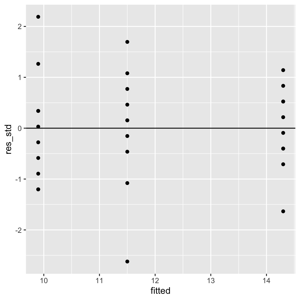
The assumption of normally distributed residuals can be checked using a QQ-plot:
ggplot(yields_residuals_fitted, aes()) +
  stat_qq(aes(sample = res_std)) +
  geom_abline(intercept = 0, slope = 1)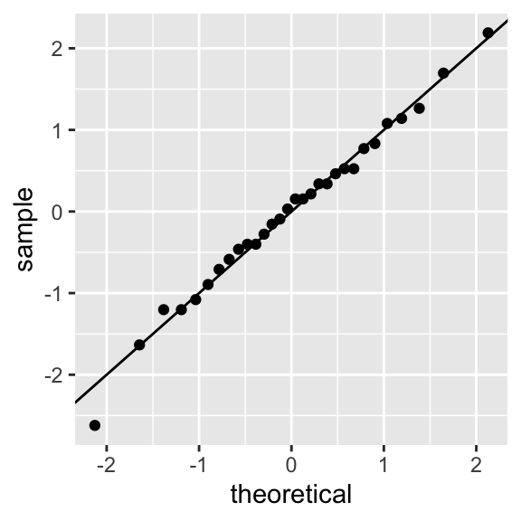
We can extract the group means using the model.tables()
function:
model.tables(soil.aov, type = "means")## Tables of means
## Grand mean
##
## 11.9
##
## soiltype
## soiltype
## clay loam sand
## 11.5 14.3 9.9Or we can extract the effect sizes, that is the differences in means, which is often more interesting:
model.tables(soil.aov, type = "effects")## Tables of effects
##
## soiltype
## soiltype
## clay loam sand
## -0.4 2.4 -2.0We already know from the ANOVA that at least two soil types have significantly different yields. However, it would be good to know which differences are significant. Therefore, we use Tukey’s ‘Honest Significant Difference’ Method:
TukeyHSD(soil.aov)## Tukey multiple comparisons of means
## 95% family-wise confidence level
##
## Fit: aov(formula = yield ~ soiltype, data = yields_tidy)
##
## $soiltype
## diff lwr upr p adj
## loam-clay 2.8 -0.9903777 6.5903777 0.1785489
## sand-clay -1.6 -5.3903777 2.1903777 0.5546301
## sand-loam -4.4 -8.1903777 -0.6096223 0.0204414Why do we need to correct for multiple testing? Let’s have a look at XKCD: https://xkcd.com/882/
By repeating an hypothesis test on the same sample, we increase our chance of making a ‘false positive’ discovery (alpha-error).
Consider a significance level of p<0.05. When doing 20 tests on the same sample, we would expect one significant result just by chance - as in the comic - even if really there is no significance.
There are several methods to correct for this issue, of which
TukeyHSD is only one (see ?p.adjust for further info).
The probability of hitting a false positive increases with the number of comparisons, which is not only determined by the number of tests, but also the number of data-processing steps you perform. This problem is known as the Garden of Forking Pathes (Gelman and Loken 2013).
We can plot the differences in means (effect sizes) using points and error bars:
tukey <- as.data.frame(TukeyHSD(soil.aov)$soiltype)
tukey$soiltype <- rownames(tukey)

ggplot(tukey, aes(x = soiltype, y = diff)) +
  geom_point() +
  geom_errorbar(aes(ymin = lwr, ymax = upr), width = 0.25) +
  geom_hline(yintercept = 0) +
  labs(x = "Soiltype", y = "Differnece in means")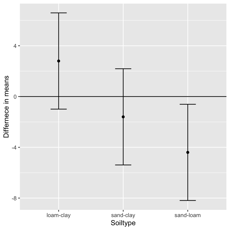
Crawley, M. J. 2012. The R Book (2nd Ed.). Chichester: John Wiley & Sons Ltd.
Copyright © 2024 Humboldt-Universität zu Berlin. Department of Geography.
![]()