Content
- Log-linear regression: count response data (Poisson model with log-link)
- Over-dispersion: quasi-Poisson model
- Over-dispersion: negative-binomial model
The following data set shows bird counts over a topographic relief gradient:
dat <- read.table("Data/bird_counts.txt", sep = ";", header = TRUE)
head(dat)
## relief Y
## 1 0.576 129
## 2 0.576 166
## 3 0.576 137
## 4 0.576 105
## 5 0.576 155
## 6 0.576 178ggplot(dat, aes(x = relief, y = Y)) +
geom_point()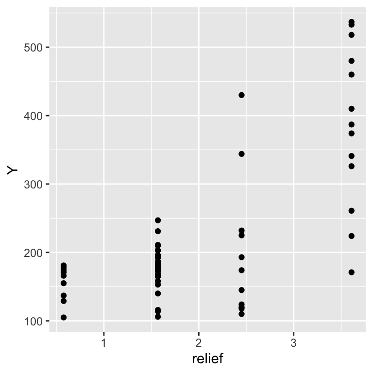
ggplot(dat, aes(x = relief, y = Y)) + scale_y_continuous(trans='log') +
  geom_point()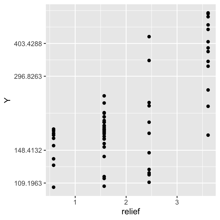
The data is bounded to positive values, a log-link is thus recommended:
countsexpected=log−1(β0+β1∗relief)=exp(β0+β1∗relief)
As the data can only take natural numbers (0, 1, 2, …), we need a discrete response distribution. For count data, the Poisson distribution is a good choice, yielding the final model of:
counts∼Poisson(exp(β0+β1∗relief))
bird.poisson <- glm(Y ~ relief, data = dat, family = poisson(link = "log"))summary(bird.poisson) ##
## Call:
## glm(formula = Y ~ relief, family = poisson(link = "log"), data = dat)
##
## Coefficients:
## Estimate Std. Error z value Pr(>|z|)
## (Intercept) 4.665888 0.021577 216.24 <2e-16 ***
## relief 0.339559 0.008382 40.51 <2e-16 ***
## ---
## Signif. codes: 0 '***' 0.001 '**' 0.01 '*' 0.05 '.' 0.1 ' ' 1
##
## (Dispersion parameter for poisson family taken to be 1)
##
## Null deviance: 2921.1 on 60 degrees of freedom
## Residual deviance: 1299.6 on 59 degrees of freedom
## AIC: 1739.7
##
## Number of Fisher Scoring iterations: 4Dispersion quantifies, how much higher (or lower) the observed variance is relative to the expected variance of the model.
For the Poisson distribution, the expected value is equal to the variance, i.e. the variance increases 1:1 with the mean value. Hence, dispersion = 1.
In other words, when we fit a Poisson model, we expect the variance to increase with the mean value by a factor of 1.
If the variance decreases at a lower rate, then the data are under-dispersed
If the variance decreases at a higher rate, then the data are over-dispersed. This is often the case.
With a correct mean model we have consistent estimates of the parameters but over-dispersion leads to:
underestimation of the standard errors of the parameter estimates
selection of overly complex models
To get a rough estimate on over-dispersion, divide the residual deviance by the residual degree’s of freedom. The ratio should be below 1. Values much larger (> 2) indicate over-dispersion (or under-dispersion if less than 0.6).
## Residual deviance: 1299.6  on 59  degrees of freedom
summary(bird.poisson)$deviance / summary(bird.poisson)$df.residual
## [1] 22.02709Our model appears to be over-dispersed, indicating:
bad model fit (omitted terms/variables, incorrect relationship/link, outliers)
the variation of Y is greater than predicted by the model
Remedy:
Change distribution/link-function
Change optimization (quasi-likelihood)
In the quasi-poisson regression, the variance is assumed to be a linear function of the mean.
bird.quasip <- glm(Y ~ relief, data = dat, family = quasipoisson)
summary(bird.quasip)
##
## Call:
## glm(formula = Y ~ relief, family = quasipoisson, data = dat)
##
## Coefficients:
## Estimate Std. Error t value Pr(>|t|)
## (Intercept) 4.66589 0.09953 46.878 < 2e-16 ***
## relief 0.33956 0.03866 8.782 2.64e-12 ***
## ---
## Signif. codes: 0 '***' 0.001 '**' 0.01 '*' 0.05 '.' 0.1 ' ' 1
##
## (Dispersion parameter for quasipoisson family taken to be 21.27853)
##
## Null deviance: 2921.1 on 60 degrees of freedom
## Residual deviance: 1299.6 on 59 degrees of freedom
## AIC: NA
##
## Number of Fisher Scoring iterations: 4In the negative-binomial regression, the variance is assumed to be a quadratic function of the mean, modulated by an additional variance parameter.
library(MASS)##
## Attaching package: 'MASS'## The following object is masked from 'package:dplyr':
##
## selectbird.nb <- glm.nb(Y ~ relief, data = dat, link = log)
summary(bird.nb) ##
## Call:
## glm.nb(formula = Y ~ relief, data = dat, link = log, init.theta = 11.71533906)
##
## Coefficients:
## Estimate Std. Error z value Pr(>|z|)
## (Intercept) 4.72453 0.08796 53.714 < 2e-16 ***
## relief 0.31269 0.03893 8.032 9.59e-16 ***
## ---
## Signif. codes: 0 '***' 0.001 '**' 0.01 '*' 0.05 '.' 0.1 ' ' 1
##
## (Dispersion parameter for Negative Binomial(11.7153) family taken to be 1)
##
## Null deviance: 134.313 on 60 degrees of freedom
## Residual deviance: 61.519 on 59 degrees of freedom
## AIC: 681.88
##
## Number of Fisher Scoring iterations: 1
##
##
## Theta: 11.72
## Std. Err.: 2.21
##
## 2 x log-likelihood: -675.879The coefficients of all above models can be interpreted easily, as
the coefficients are multiplicative when back-transformed to the
response (count) scale. That is, with a one unit increase in x, the
count is multiplied by the exponential of the coefficient. For our
example, we expect a 1.4 times (or 40%) increase in mean bird counts
with a one unit increase in relief. You can use confint()
to compute confidence intervals for the parameters.
# Poisson
coeffs <- exp(coef(bird.poisson))
coeffs_ci <- exp(confint(bird.poisson))
cbind(coeffs, coeffs_ci)
## coeffs 2.5 % 97.5 %
## (Intercept) 106.259866 101.846790 110.836066
## relief 1.404328 1.381446 1.427589# quasi-Poisson
coeffs <- exp(coef(bird.quasip))
coeffs_ci <- exp(confint(bird.quasip))
cbind(coeffs, coeffs_ci)## coeffs 2.5 % 97.5 %
## (Intercept) 106.259866 87.187307 128.808562
## relief 1.404328 1.301813 1.514927# negative-binomial
coeffs <- exp(coef(bird.nb))
coeffs_ci <- exp(confint(bird.nb))
cbind(coeffs, coeffs_ci) ## coeffs 2.5 % 97.5 %
## (Intercept) 112.677003 95.549671 133.298947
## relief 1.367104 1.271319 1.471155pseudo-r2=1−residual devianceNull deviance
pseudo_r2 <- 1 - bird.quasip$deviance / bird.quasip$null.deviance
pseudo_r2
## [1] 0.5551062efct <- effect("relief", mod = bird.quasip, xlevels = list(relief = seq(0, 4, length.out = 100)))
efct <- as.data.frame(efct)
p <- ggplot() +
geom_point(data = dat, aes(x = relief, y = Y)) +
geom_ribbon(data = efct, aes(x = relief, ymin = lower, ymax = upper), alpha = 0.3) +
geom_line(data = efct, aes(x = relief, y = fit))
print(p)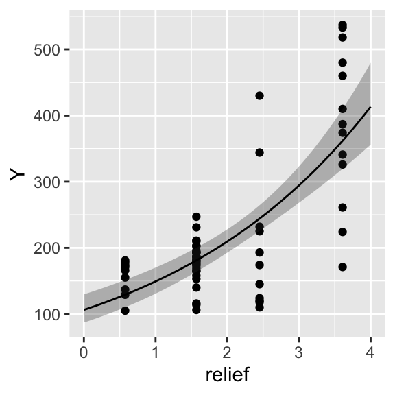
library(gridExtra)
plot1 <- ggplot(dat, aes(x = relief, y = Y)) +
                geom_point() +
                geom_smooth(method = "glm", method.args=list(family = "poisson"), col = "red")

plot2 <- ggplot(dat, aes(x = relief, y = Y)) +
                geom_point() +
                geom_smooth(method = "glm", method.args=list(family = "quasipoisson"), col = "red")

grid.arrange(plot1, plot2, ncol = 2)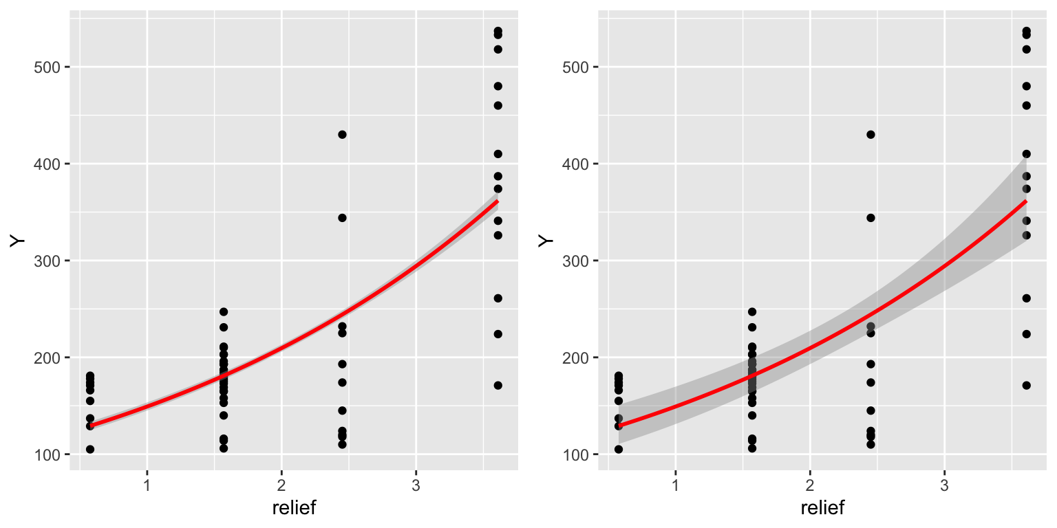
plot3 <- ggplot(dat, aes(x = relief, y = Y)) +
                geom_point() +
                geom_smooth(method = "glm.nb", method.args=list(link = "log"), col = "red")

grid.arrange(plot1, plot2, plot3, ncol = 3)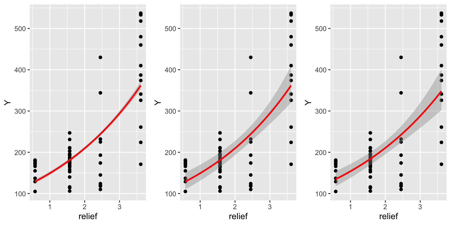
Copyright © 2024 Humboldt-Universität zu Berlin. Department of Geography.
![]()