- Packages
- Data
- Meteorological data
- DEM
- Country boundary
- The
sfpackage
- Read a spatial vector dataset
- Subset features
- Visualize features
- Create a spatial data.frame
- Coordinate reference systems
- sf and ggplot
- Interactive visualization
- Extract raster values
- Rasterize vectors
- Conversion to
sp
- Reading
Spatial Vectors in R
Humboldt-Universität zu Berlin | Geography Department
Packages
library(terra)      # Reading and manipulating raster data
library(sf)         # Reading and manipulating vector data
library(mapview)    # Map visualization
library(ggplot2)    # Visualization
library(dplyr)      # Manipulate data.frames
mapviewOptions(fgb = FALSE)
Data
Meteorological data
For this exercise we will use long-term average climate station data
from the German Meteorological Service (DWD, Climate Data Center). Monthly,
annual, and multi-annual
meteorological data are available for different time periods. Here, we
have multi-annual precipitation (mm) data for individual months and the
entire year (column year) for the period 1981 and 2010. The
dataset contains coordinates in geographic longitude (x)
and latitude (y) (EPSG:
4326).
precp_df <- read.csv('data/nieder_1981-2010_aktStandort.csv')
head(precp_df[, -10:-15])
## station_name station_id elevation y x state jan feb mar oct nov dec year
## 1 AACHEN-ORSBACH 15000 231 51 6.0 Nordrhein-Westfalen 78 72 72 74 73 84 914
## 2 ABBENSEN 12 61 52 10.2 Niedersachsen 60 46 56 53 56 64 697
## 3 AFFING 37 470 48 11.0 Bayern 46 42 54 56 54 59 817
## 4 AHAUS(AWST) 7374 46 52 6.9 Nordrhein-Westfalen 78 61 70 71 76 81 852
## 5 AHAUSEN 39 29 53 9.3 Niedersachsen 72 54 64 67 66 73 788
## 6 AHLEN I_W_ 42 70 52 7.9 Nordrhein-Westfalen 68 52 64 64 66 70 770DEM
Further, we’ll use a digital elevation model from the Copernicus Land Services downsampled to 1 x 1km. The coordinate reference system (projection) is a Lambert Azimuthal Equal Area Projection for Europe (EPSG:3035).
dem <- rast('data/eu_dem_v11_de_1km.tif')
plot(dem)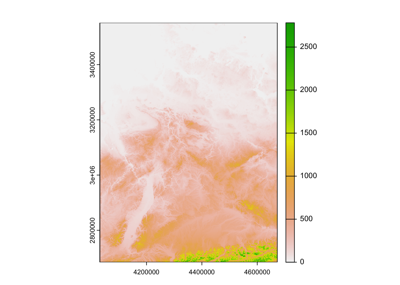
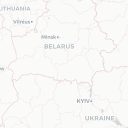
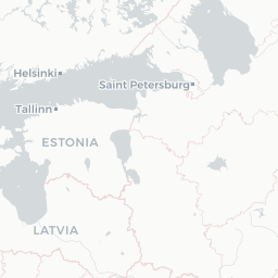
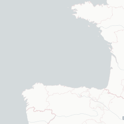
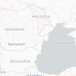
Country boundary
To facilitate the visual interpretation of the output maps, we’ll use
the boundaries of selected European countries stored in a Geopackage.
The coordinate reference system (projection) is also Lambert Azimuthal
Equal Area Projection for Europe (EPSG:3035):
data/cntry_boundary_europe-subset.gpkg.
The sf package
The sf package provides classes to read, write, and
manipulate vector data in R (Pebesma,
2018). The sf package supersedes the older
sp package. Because the sp package has been
around for a longer time, dependencies with some packages may still
exist. But development of sp will eventually be stopped at
some point. The letters sf stand for ‘simple features’ or ‘simple
feature access’, which is a formal standard that will make handling and
conversion of vector data easier.
The sf package represents simple features as native R
objects, using simple data structures (S3 classes, lists, matrices,
vectors). All functions and methods in sf that operate on
spatial data are prefixed by st_, which refers to spatial
and temporal.
In the sf package three classes are used to represent
simple features:
sf: a spatial data.frame with feature attributes and feature geometries. The geometry column is of classsfcand is typically called geometry or geom but any name can be used.sfc: the list-column with the geometries for each feature (record), which is composed ofsfg.sfg: the feature geometry of an individual simple feature, e.g. a point, linestring, multilinestring, polygon, multipolygon.
Read a spatial vector dataset
The function read_sf() can be used to read a spatial
vector dataset in memory. read_sf() is an alias to
st_read() to be consistent with other read functions in R
(recall all sf functions start with st_).
cntry <- read_sf('data/cntry_boundary_europe-subset.gpkg')
head(cntry)
## Simple feature collection with 6 features and 6 fields
## Geometry type: MULTIPOLYGON
## Dimension: XY
## Bounding box: xmin: 3600000 ymin: 1900000 xmax: 5800000 ymax: 3800000
## Projected CRS: ETRS89-extended / LAEA Europe
## # A tibble: 6 × 7
## COUNTRY ISO_CC CONTINENT Land_Type Land_Rank COUNTRYAFF geom
## <chr> <chr> <chr> <chr> <int> <chr> <MULTIPOLYGON [m]>
## 1 Albania AL Europe Primary la… 5 Albania (((5150486 2214643, 5156…
## 2 Andorra AD Europe Primary la… 5 Andorra (((3640340 2192709, 3638…
## 3 Austria AT Europe Primary la… 5 Austria (((4832066 2857840, 4832…
## 4 Belarus BY Europe Primary la… 5 Belarus (((5787402 3444248, 5784…
## 5 Belgium BE Europe Primary la… 5 Belgium (((4e+06 3079060, 4e+06 …
## 6 Bosnia and Herzegovina BA Europe Primary la… 5 Bosnia an… (((5e+06 2459212, 5e+06 …The country dataset is a multipolygon vector dataset with the
attributes: COUNTRY, ISO_CC, CONTINENT, Land_Type and geom (the geometry
column). The geometry column is of class sfc.
class(cntry$geom)## [1] "sfc_MULTIPOLYGON" "sfc"Subset features
The spatial data.frame acts in many ways like an ordinary data.frame.
We can subset feature sets by using the square bracket notation. Below I
subset the feature set to only include the boundary of Germany (rows)
and the feature attribute ISO_CC (columns).
cntry_de <- cntry[cntry$COUNTRY=="Germany", "ISO_CC"]Similarly, the dplyr functions work on sf objects as
well.
cntry_de <- dplyr::filter(cntry, COUNTRY=="Germany")Visualize features
The basic plot() function works with sf
objects. If you use plot() all feature attributes are
plotted. For more information see: https://r-spatial.github.io/sf/articles/sf5.html
plot(cntry, max.plot=4)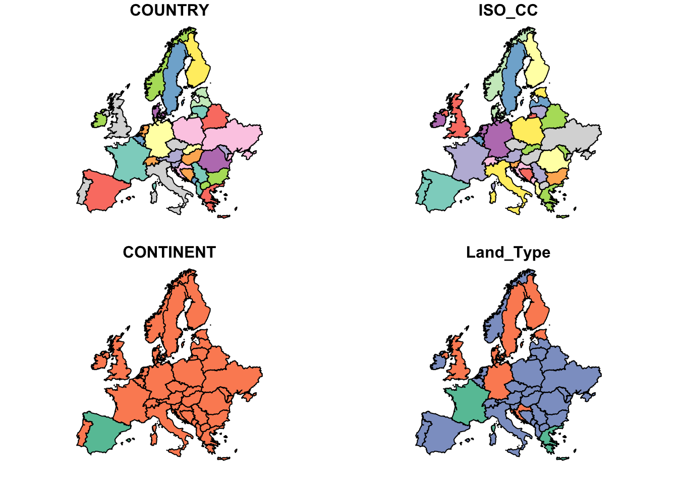
Subset the dataset using square brackets to visualize only one (or selected) feature attributes:
plot(cntry["COUNTRY"])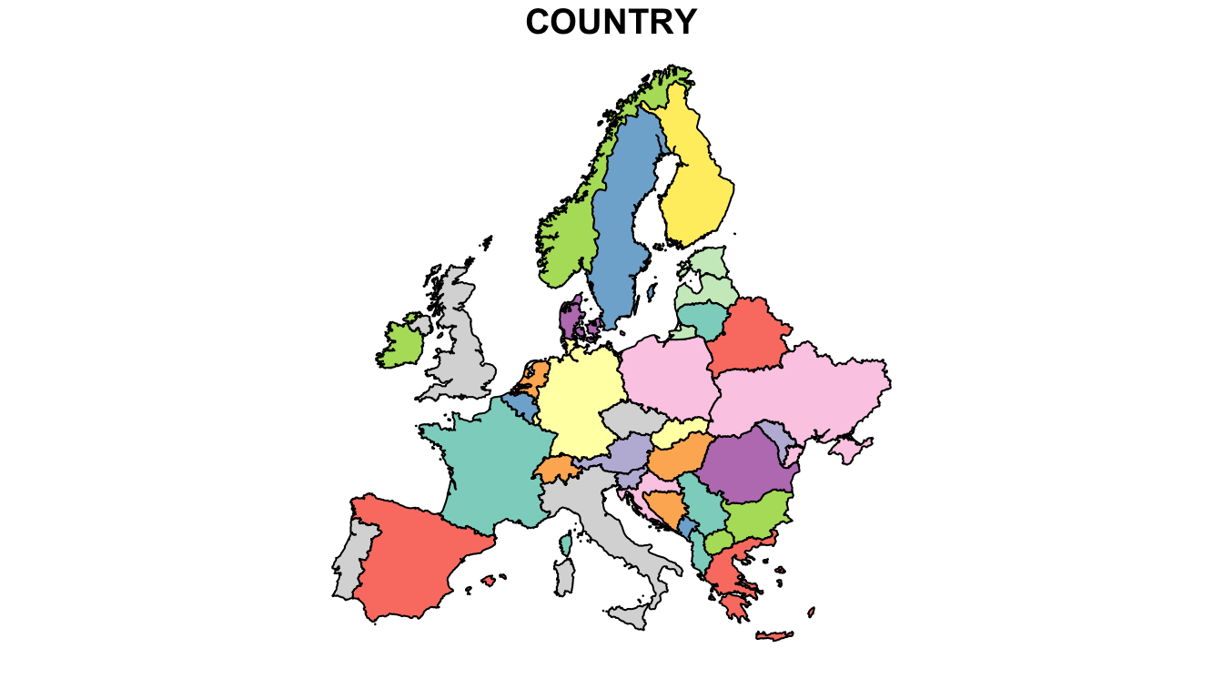
It is also possible to only plot the geometry.
plot(st_geometry(cntry))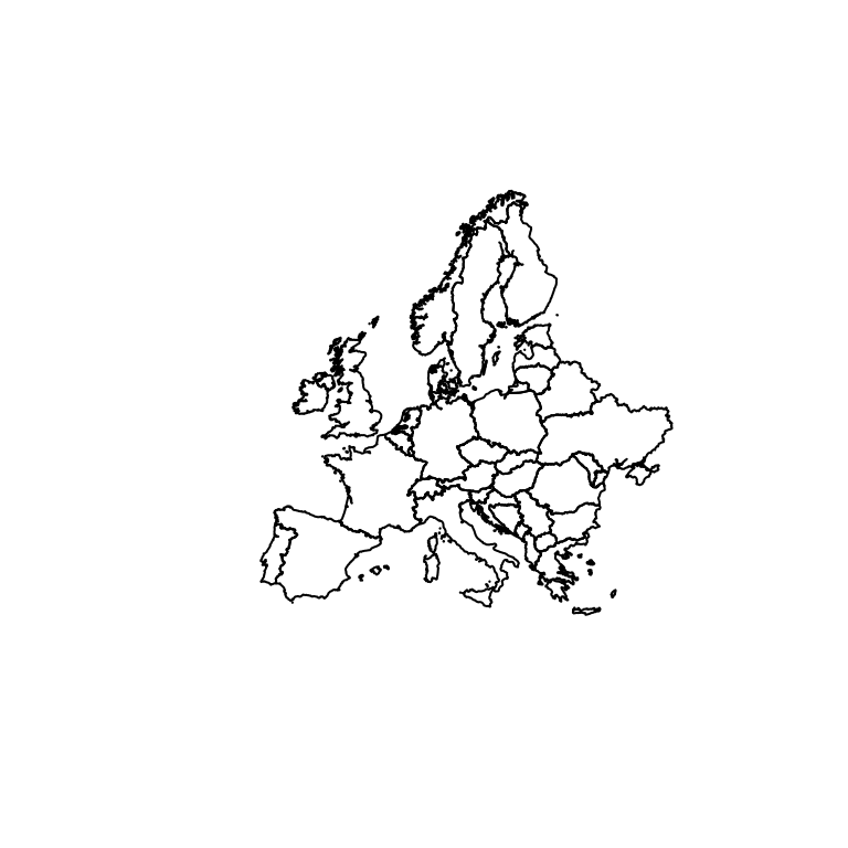
Create a spatial data.frame
We can convert our precipitation data.frame into a spatial data.frame
(sf object) using the function st_as_sf(). To
define the coordinate reference system (crs), we can use
the epsg code
for the geographic coordinate system in WGS84, but other specifications
like the proj4
string also work. The coordinates are supplied via the function
argument coords, either as a vector of the names in the
data.frame that contain the coordinates, or as a matrix that contains
the coordinates. In our case, the precipitation data.frame contains a
column x and y.
precp_geo <- st_as_sf(precp_df, coords=c('x','y'), crs=4326)
precp_geo[, -9:-16]
## Simple feature collection with 874 features and 9 fields
## Geometry type: POINT
## Dimension: XY
## Bounding box: xmin: 6 ymin: 47 xmax: 15 ymax: 55
## Geodetic CRS: WGS 84
## First 10 features:
## station_name station_id elevation state jan feb mar apr year geometry
## 1 AACHEN-ORSBACH 15000 231 Nordrhein-Westfalen 78 72 72 59 914 POINT (6 51)
## 2 ABBENSEN 12 61 Niedersachsen 60 46 56 42 697 POINT (10 52)
## 3 AFFING 37 470 Bayern 46 42 54 54 817 POINT (11 48)
## 4 AHAUS(AWST) 7374 46 Nordrhein-Westfalen 78 61 70 48 852 POINT (6.9 52)
## 5 AHAUSEN 39 29 Niedersachsen 72 54 64 44 788 POINT (9.3 53)
## 6 AHLEN I_W_ 42 70 Nordrhein-Westfalen 68 52 64 44 770 POINT (7.9 52)
## 7 AHORN-EUBIGHEIM 47 338 Baden-Württemberg 64 56 66 51 783 POINT (9.6 50)
## 8 ALBERSDORF 66 40 Schleswig-Holstein 76 59 66 46 939 POINT (9.3 54)
## 9 ALBSTADT-BADKAP 71 759 Baden-Württemberg 68 64 79 72 1014 POINT (9 48)
## 10 ALFELD (AWST) 7367 144 Niedersachsen 83 64 74 54 877 POINT (9.8 52)Coordinate reference systems
The function st_crs() is used to access or define the
coordinate reference system.
st_crs(precp_geo)## Coordinate Reference System:
## User input: EPSG:4326
## wkt:
## GEOGCRS["WGS 84",
## DATUM["World Geodetic System 1984",
## ELLIPSOID["WGS 84",6378137,298.257223563,
## LENGTHUNIT["metre",1]]],
## PRIMEM["Greenwich",0,
## ANGLEUNIT["degree",0.0174532925199433]],
## CS[ellipsoidal,2],
## AXIS["geodetic latitude (Lat)",north,
## ORDER[1],
## ANGLEUNIT["degree",0.0174532925199433]],
## AXIS["geodetic longitude (Lon)",east,
## ORDER[2],
## ANGLEUNIT["degree",0.0174532925199433]],
## USAGE[
## SCOPE["Horizontal component of 3D system."],
## AREA["World."],
## BBOX[-90,-180,90,180]],
## ID["EPSG",4326]]We can also (re-)assign a coordinate reference system. Note, this does not reproject the dataset.
st_crs(precp_geo) <- 4326Using st_transform(), we can reproject the spatial
data.frame to another coordinate system. Here, we repoject it to the
same coordinate reference system as the DEM.
precp_laea <- st_transform(precp_geo, 3035)
st_crs(precp_laea)
## Coordinate Reference System:
## User input: EPSG:3035
## wkt:
## PROJCRS["ETRS89-extended / LAEA Europe",
## BASEGEOGCRS["ETRS89",
## ENSEMBLE["European Terrestrial Reference System 1989 ensemble",
## MEMBER["European Terrestrial Reference Frame 1989"],
## MEMBER["European Terrestrial Reference Frame 1990"],
## MEMBER["European Terrestrial Reference Frame 1991"],
## MEMBER["European Terrestrial Reference Frame 1992"],
## MEMBER["European Terrestrial Reference Frame 1993"],
## MEMBER["European Terrestrial Reference Frame 1994"],
## MEMBER["European Terrestrial Reference Frame 1996"],
## MEMBER["European Terrestrial Reference Frame 1997"],
## MEMBER["European Terrestrial Reference Frame 2000"],
## MEMBER["European Terrestrial Reference Frame 2005"],
## MEMBER["European Terrestrial Reference Frame 2014"],
## ELLIPSOID["GRS 1980",6378137,298.257222101,
## LENGTHUNIT["metre",1]],
## ENSEMBLEACCURACY[0.1]],
## PRIMEM["Greenwich",0,
## ANGLEUNIT["degree",0.0174532925199433]],
## ID["EPSG",4258]],
## CONVERSION["Europe Equal Area 2001",
## METHOD["Lambert Azimuthal Equal Area",
## ID["EPSG",9820]],
## PARAMETER["Latitude of natural origin",52,
## ANGLEUNIT["degree",0.0174532925199433],
## ID["EPSG",8801]],
## PARAMETER["Longitude of natural origin",10,
## ANGLEUNIT["degree",0.0174532925199433],
## ID["EPSG",8802]],
## PARAMETER["False easting",4321000,
## LENGTHUNIT["metre",1],
## ID["EPSG",8806]],
## PARAMETER["False northing",3210000,
## LENGTHUNIT["metre",1],
## ID["EPSG",8807]]],
## CS[Cartesian,2],
## AXIS["northing (Y)",north,
## ORDER[1],
## LENGTHUNIT["metre",1]],
## AXIS["easting (X)",east,
## ORDER[2],
## LENGTHUNIT["metre",1]],
## USAGE[
## SCOPE["Statistical analysis."],
## AREA["Europe - European Union (EU) countries and candidates. Europe - onshore and offshore: Albania; Andorra; Austria; Belgium; Bosnia and Herzegovina; Bulgaria; Croatia; Cyprus; Czechia; Denmark; Estonia; Faroe Islands; Finland; France; Germany; Gibraltar; Greece; Hungary; Iceland; Ireland; Italy; Kosovo; Latvia; Liechtenstein; Lithuania; Luxembourg; Malta; Monaco; Montenegro; Netherlands; North Macedonia; Norway including Svalbard and Jan Mayen; Poland; Portugal including Madeira and Azores; Romania; San Marino; Serbia; Slovakia; Slovenia; Spain including Canary Islands; Sweden; Switzerland; Türkiye (Turkey); United Kingdom (UK) including Channel Islands and Isle of Man; Vatican City State."],
## BBOX[24.6,-35.58,84.73,44.83]],
## ID["EPSG",3035]]sf and ggplot
The sf package also provides functions like
geom_sf() to work with ggplot(). In the map
below, we display the annual precipitation, which is stored in the
feature attribute year. You see, the map is in in
geographic latitude/longitude by default. You can change the coordinate
reference system of the map with coord_sf().
ggplot() +
  geom_sf(data=precp_laea, aes(col=year)) +
  geom_sf(data=st_geometry(cntry_de), fill=NA) # + coord_sf(datum = st_crs(3035))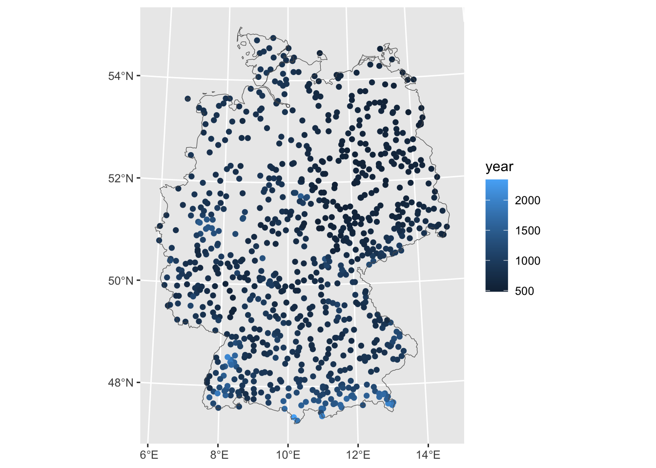
Interactive visualization
The mapview package provides a convenient way to visualize geodata interactively on top of different base maps such as OpenStreetMap.
mapview(precp_laea["year"])


Extract raster values
We can extract raster attributes for vector features using the
extract() function from the terra packages.
Here, we extract elevation from the Copernicus DEM at every
meteorological station. Note, the precipitation data already contains an
elevation attribute. You can compare the two values if you like.
elev1k <- terra::extract(dem, precp_laea)
head(elev1k)
## ID eu_dem_v11_de_1km
## 1 1 205
## 2 2 64
## 3 3 484
## 4 4 44
## 5 5 21
## 6 6 76Add extracted values to the precipitation data.frame.
precp_laea$elev1k <- elev1k[,2] # remove ID column
head(precp_laea)
## Simple feature collection with 6 features and 18 fields
## Geometry type: POINT
## Dimension: XY
## Bounding box: xmin: 4e+06 ymin: 2800000 xmax: 4400000 ymax: 3300000
## Projected CRS: ETRS89-extended / LAEA Europe
## station_name station_id elevation state jan feb mar apr mai jun jul aug sept oct
## 1 AACHEN-ORSBACH 15000 231 Nordrhein-Westfalen 78 72 72 59 77 89 80 82 74 74
## 2 ABBENSEN 12 61 Niedersachsen 60 46 56 42 55 67 68 73 57 53
## 3 AFFING 37 470 Bayern 46 42 54 54 90 92 106 96 68 56
## 4 AHAUS(AWST) 7374 46 Nordrhein-Westfalen 78 61 70 48 65 74 77 76 75 71
## 5 AHAUSEN 39 29 Niedersachsen 72 54 64 44 58 70 80 73 67 67
## 6 AHLEN I_W_ 42 70 Nordrhein-Westfalen 68 52 64 44 63 65 71 69 74 64
## nov dec year geometry elev1k
## 1 73 84 914 POINT (4e+06 3084134) 205
## 2 56 64 697 POINT (4333483 3252669) 64
## 3 54 59 817 POINT (4393745 2817509) 484
## 4 76 81 852 POINT (4110850 3223695) 44
## 5 66 73 788 POINT (4275191 3328909) 21
## 6 66 70 770 POINT (4173751 3186191) 76Rasterize vectors
The rasterize() function of the terra
package can be used to turn spatial vectors into rasters. When
rasterizing point vectors, a function is applied to all points falling
into a grid cell. For example the function length() counts
the number of points in a grid cell.
The rasterize() function requires a template raster as
input. The template raster can be an existing, valid raster or an empty
raster (no cell values). Here, we use the DEM raster as template, but
change the spatial resolution to 20 km x 20 km. Note, we loose the pixel
values, when we simply change the spatial resolution like that. But that
is OK for a template.
template <- dem
res(template) <- c(20000, 20000)
To feed the terra package a spatial vector dataset, we
need to convert the sf object into a
SpatVector object using the vect() function.
The argument fun takes either the name of a built-in
functions or a function object. Let’s create two rasters:
countgrid contains the the number of stations in each grid
cell and meangrid contains the mean annual precipitation
(field=year).
countgrid <- terra::rasterize(vect(precp_laea), template, fun = "length", background = NA)
meangrid <- terra::rasterize(vect(precp_laea), template, field="year", fun = "mean", background = NA)

# To add the country boundary to mutiple subplots, we need to put the line of
# code where we add the country boundary into a separate function.
add_boundary <- function() plot(st_geometry(cntry_de), add=T)

plot(c(countgrid, meangrid),
     main=c("Count", "Mean annual precipitation"),
     fun=add_boundary)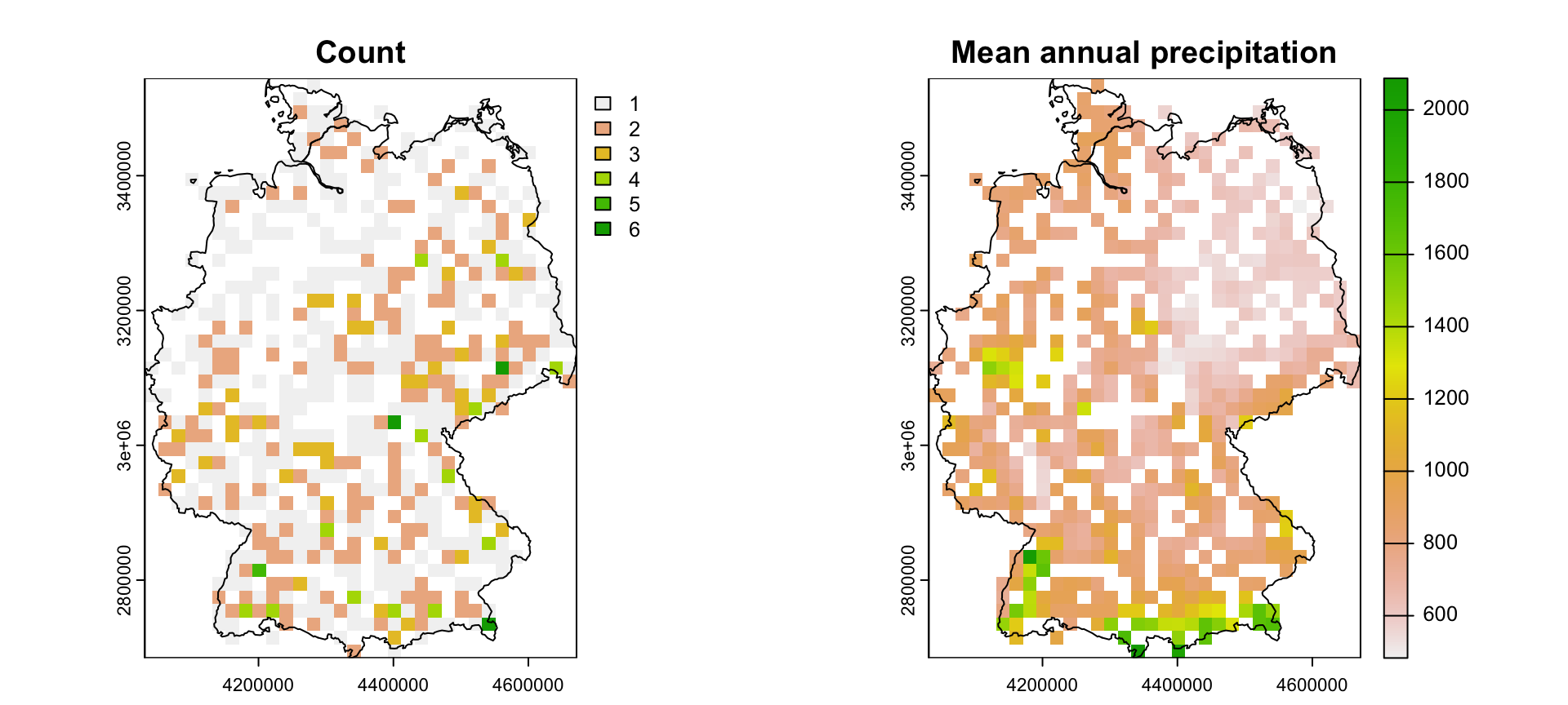
Conversion to sp
Spatial objects from the outdated sp package can be
converted into simple feature objects or geometries using
st_as_sf() and st_as_sfc(), respectively.
Conversely, simple feature objects can be converted into sp
objects using the as() function as follows:
library(sp)

precp_sp <- as(precp_laea, "Spatial")
class(precp_sp)
## [1] "SpatialPointsDataFrame"
## attr(,"package")
## [1] "sp"Reading
Copyright © 2024 Humboldt-Universität zu Berlin. Department of Geography.
![]()