Content

From LM to GLM
The GLM in R
Logistic regression: proportions response data
Logistic regression: binary response data

Generalized Linear Models

In the linear model, the mean response \(E[y_i]\) is modelled by a linear function of explanatory variables \(x_{ik}\) plus a residual term \(\epsilon_i\),

\[\begin{aligned}E[y_i] + \epsilon_i = \beta_{0} + \beta_{1} x_{i1} + ... + \beta_{k} x_{ik} + \epsilon_i\end{aligned}\]
where \(i\) is the observation index and \(k\) is the index of explanatory variables.

We assume that the residuals \(\epsilon_i\) are independent and identically distributed according to a normal distribution such that

\[\begin{aligned} E(\epsilon_i) = 0 \\ Var(\epsilon_i) = \sigma^2 \end{aligned}\]

The random residual term can also be written as

\[\begin{aligned} \epsilon_i \sim N(0, \sigma)\end{aligned}\]

This can also be written in terms of \(y_i\), with the linear predictor as the mean response and variance \(\sigma^2\) (standard deviation \(\sigma\)).

\[\begin{aligned} y_i \sim N(E[y_i], \sigma)\end{aligned}\]

We now extend this case to different distributional assumptions, which also involves transformations of the linear predictor to fit into those distributions.

The `glm` function

These are Generalized Linear Models that can be fitted in R using the glm function, which is similar to the lm function for fitting linear models. The arguments to a glm call are as follows

glm(formula, family = gaussian, data, weights, subset, na.action, start = NULL, etastart, mustart, offset, control = glm.control(...), model = TRUE, method = ”glm.fit”, x = FALSE, y = TRUE, contrasts = NULL, ...)

Family argument

The family argument takes (the name of) a family function which specifies

the distributional assumption
the link function

The exponential family functions available in R are

binomial(link = "logit")
gaussian(link = "identity")
Gamma(link = "inverse")
inverse.gaussian(link = "1/mu2")
poisson(link = "log")

The link functions listed are the default choices, but you can - in principle - mix and match if you have reason to do so.

Extractor functions

The glm function returns an object of class c(“glm”, “lm”). There are several glm or lm methods available for accessing/displaying components of the glm object, including:

residuals()
fitted()
predict()
coef()
deviance()
formula()
summary()

From LM to GLM

Remember the airquality regression problem:

\[\begin{aligned}E[y_i] = \beta_{0} + \beta_{1} Temp_i + \beta_2 Wind_i + \beta_3 Temp_i Wind_i\end{aligned}\]

We found that the residuals were not well distributed, because of ozone concentration being bounded to positive values. We transformed the response to overcome this problem:

\[\begin{aligned}E[log(y_i)] = \beta_{0} + \beta_{1} Temp_i + \beta_2 Wind_i + \beta_3 Temp_i Wind_i\end{aligned}\] However, transforming the response can make the interpretation of the model challenging, as well as the back-transformation of standard errors and confidence intervals can be difficult.

The idea behind GLMs is that we transform our mean response via a so-called link-function \(g()\). Compare with the equation above. This is different to transforming individual \(y_i\)’s.

\[\begin{aligned}g(E[y_i]) = \beta_{0} + \beta_{1} Temp_i + \beta_2 Wind_i + \beta_3 Temp_i Wind_i\end{aligned}\] The linear predictor is often written as \(\eta_i\).

\(\eta_i = g(E[y_i])\)

The inverse-link function \(g()^{-1}\) is used to back-transform the equation to the mean response:

\(E[y_i] = g^{-1}(\eta_i)\)

For a simple-linear regression the link-function is the so-called identity link, that is \(\eta_i = E[y_i]\).

Further, we also have to assume a data distribution, which for linear regression is normal (“Gaussian”) with zero mean and a variance of \(\sigma^2\). The linear model can thus be written as:

\(y_i \sim N(E[y_i], \sigma)\)

Running a simple linear regression using glm() and comparing to lm() produces identical results:

fit.lm <- lm(Ozone ~ Temp * Wind, data = na.omit(airquality))

fit.glm <- glm(Ozone ~ Temp * Wind, data = na.omit(airquality), family = gaussian(link = "identity"))

coef(fit.lm)

## (Intercept)        Temp        Wind   Temp:Wind 
## -239.891827    4.000528   13.597458   -0.217276

coef(fit.glm)

## (Intercept)        Temp        Wind   Temp:Wind 
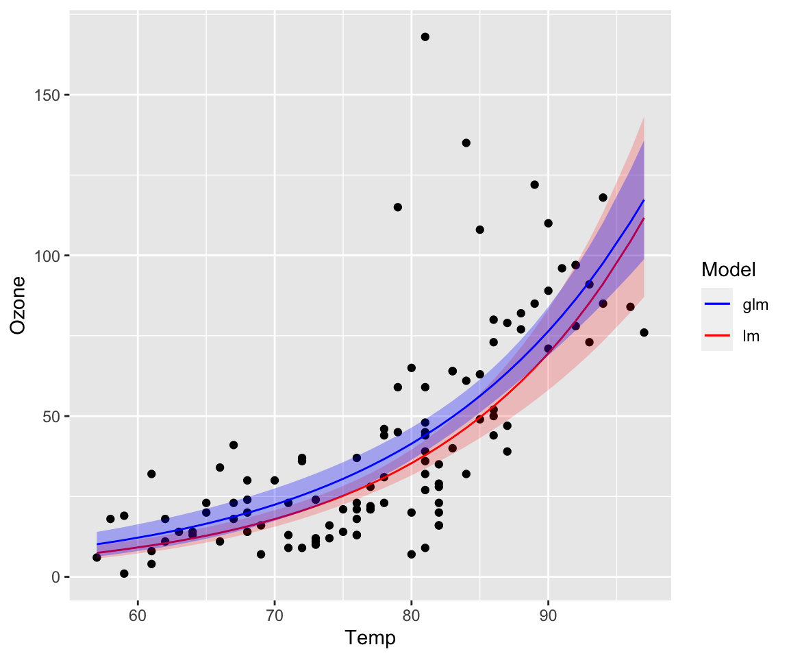
## -239.891827    4.000528   13.597458   -0.217276

Now we want to account for the non-linear relationship. Instead of transforming the response \(log(y_i)\), we now define a log link-function linking the linear predictor to the mean response \(log(E[y_i])\):

fit.glm <- glm(Ozone ~ Temp, data = na.omit(airquality), family = gaussian(link = "log"))

The link-function is \(g(E[y_i]) = log(E[y_i]) = \eta_i\) and the inverse is \(E[y_i] + g^{-1}(\eta_i) = e^{\eta_i}\). The data distribution is still assumed to be normal and the model can also be written as:

\(y_i \sim N(e^{\eta_i}, \sigma)\)

Notice the difference to a linear model with log-transformed response.

\(y_i \sim e^{N(\eta_i, \sigma)}\)

The models are not identical. Most noticeable are the larger and increasing confidence bands of the simple linear model, which comes from transforming and back-transforming the individual observations including their variance.

Advantages

Fitted values (and confidence intervals) are calculated in the original data space, not in a transformed data space
We can select any link function fitting many data problems (bounded to positive, bounded to [0,1], …)
We can specify the data distribution (think of counts, success/failure, rates, …)

Logistic Regression

Proportions response data

We make use of a new data set:

dat <- read.table("Data/logistic.txt", sep = "\t", header = TRUE)

head(dat)

##   logdose  n dead product
## 1     0.1 18    0       A
## 2     0.2 16    4       A
## 3     0.3 21    7       A
## 4     0.4 19    6       A
## 5     0.5 16    5       A
## 6     0.6 20   10       A

ggplot(dat, aes(x = logdose, y = dead / n, col = product)) +
  geom_point() +
  scale_color_brewer(palette = "Set1") # See colorbrewer.org for palettes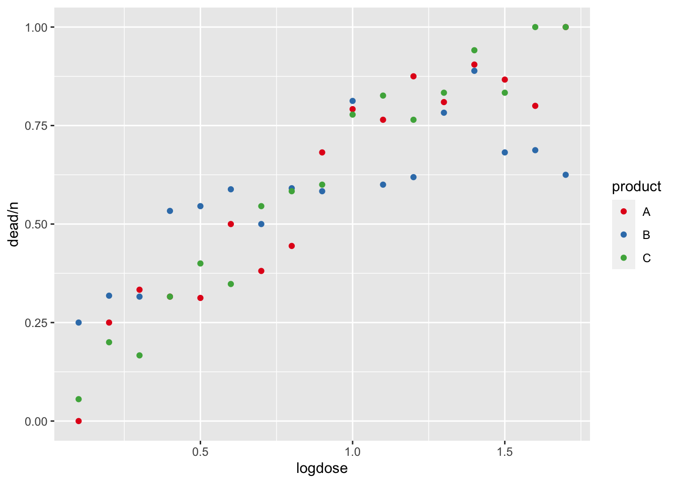

This dataset describes the number of dead cells of an organism (dead) out of an initial number of cells (n) as a function of the dose (logdose, on the log-scale) of one of three toxic substances (product).

We now aim to model the mortality-rate (bounded between 0 and 1) in response to the dose of toxin. For doing so, we need to combine the dead and surviving cells using cbind():

fit1 <- glm(cbind(dead, n - dead) ~ logdose, data = dat, family = binomial(link = "logit"))
summary(fit1)

## 
## Call:
## glm(formula = cbind(dead, n - dead) ~ logdose, family = binomial(link = "logit"), 
##     data = dat)
## 
## Coefficients:
##             Estimate Std. Error z value Pr(>|z|)    
## (Intercept)  -1.5980     0.1555  -10.27   <2e-16 ***
## logdose       2.3179     0.1699   13.64   <2e-16 ***
## ---
## Signif. codes:  0 '***' 0.001 '**' 0.01 '*' 0.05 '.' 0.1 ' ' 1
## 
## (Dispersion parameter for binomial family taken to be 1)
## 
##     Null deviance: 311.241  on 50  degrees of freedom
## Residual deviance:  72.387  on 49  degrees of freedom
## AIC: 223.39
## 
## Number of Fisher Scoring iterations: 4

As link function we choose a logit-link (bounded between 0 and 1) and we assume the data to be binomially distributed (k successes given n trials).

We can estimate the goodness of fit using pseudo-\(R^2\) (which mimics \(R^2\) of linear regression):

pseudo_r2 <- 1 - fit1$deviance / fit1$null.deviance
pseudo_r2

## [1] 0.7674258

And overlay the fitted line onto the scatter plot:

dat$fitted1 <- predict(fit1, type = "response") # Alternatively type = "link"

ggplot(dat, aes(x = logdose, y = dead/n)) +
  geom_point() +
  geom_line(data = dat, aes(x = logdose, y = fitted1))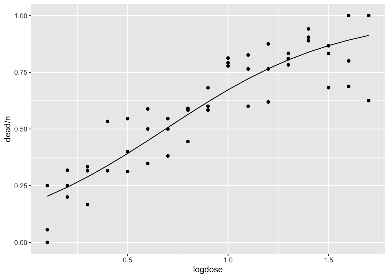

Let us see if the mortality varies by toxin:

fit2 <- glm(cbind(dead, n - dead) ~ logdose * product, data = dat, family = binomial(link = "logit"))
summary(fit2)

## 
## Call:
## glm(formula = cbind(dead, n - dead) ~ logdose * product, family = binomial(link = "logit"), 
##     data = dat)
## 
## Coefficients:
##                  Estimate Std. Error z value Pr(>|z|)    
## (Intercept)       -2.0410     0.3034  -6.728 1.72e-11 ***
## logdose            2.8768     0.3432   8.383  < 2e-16 ***
## productB           1.2920     0.3845   3.360  0.00078 ***
## productC          -0.3079     0.4308  -0.715  0.47469    
## logdose:productB  -1.6457     0.4220  -3.899 9.65e-05 ***
## logdose:productC   0.4318     0.4898   0.882  0.37793    
## ---
## Signif. codes:  0 '***' 0.001 '**' 0.01 '*' 0.05 '.' 0.1 ' ' 1
## 
## (Dispersion parameter for binomial family taken to be 1)
## 
##     Null deviance: 311.241  on 50  degrees of freedom
## Residual deviance:  42.305  on 45  degrees of freedom
## AIC: 201.31
## 
## Number of Fisher Scoring iterations: 4

Estimate the goodness of fit using pseudo-\(R^2\):

pseudo_r2 <- 1 - fit2$deviance / fit2$null.deviance
pseudo_r2

## [1] 0.8640758

Overlay this model onto the scatter plot:

library(effects)

dat.effects <- effect("logdose:product", mod = fit2, xlevels = list(logdose = seq(0, 2, length.out = 100)))
dat.effects <- as.data.frame(dat.effects)

ggplot() +
  geom_point(data = dat, aes(x = logdose, y = dead/n, col = product)) +
  geom_ribbon(data = dat.effects, aes(x = logdose, ymin = lower, ymax = upper, fill = product), alpha = 0.2) +
  geom_line(data = dat.effects, aes(x = logdose, y = fit, col = product)) +
  scale_fill_brewer(palette = "Set1") +
  scale_color_brewer(palette = "Set1")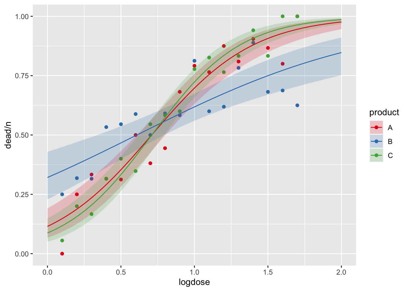

Residual analysis

Several kinds of residuals can be defined for GLMs:

response: \(r_i = y_i - E[y_i]\)
Pearson (\(r_i\) divided by square root of the variance function)
deviance

These kinds of residuals are all equivalent for normal models.

We can check the residuals using the residuals() function or rstandard() functions.

Model fit1: formula = cbind(dead, n - dead) ~ logdose

plot(fit1$fitted.values, rstandard(fit1, type = 'pearson'))
abline(h=0)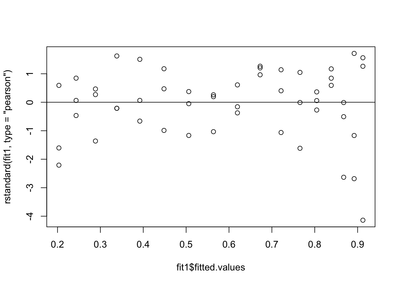

Model fit2: formula = cbind(dead, n - dead) ~ logdose * product

plot(fit2$fitted.values, rstandard(fit1, type = 'pearson'))
abline(h=0)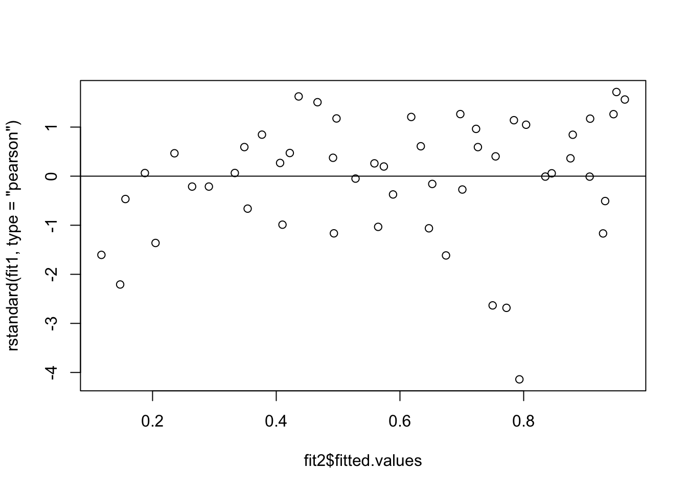

Binary response data

We now use a dataset where the response can only take two values. These data indicate whether trees were infested by a bark beetle or not, depending on the temperature anomaly (z-transformed temperatures with values > 0 indicating hotter than average):

dat <- read.csv("Data/infestation.csv")
head(dat)

##   infested temp_anomaly
## 1        1   -1.0785729
## 2        1    1.2728951
## 3        1    1.8699789
## 4        1    0.6327722
## 5        0    0.3342014
## 6        1    0.8407184

ggplot(dat, aes(x = temp_anomaly, y = infested)) +
  geom_point()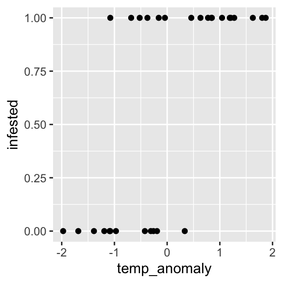

Similar problems include: dead/alive, presence/absence, conversion/conservation, etc.

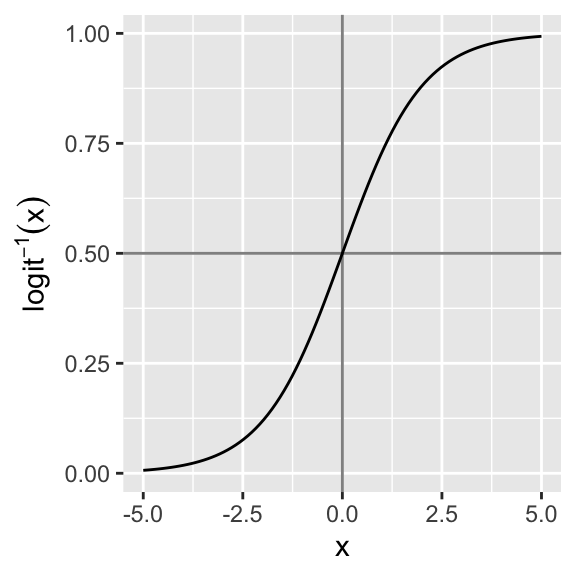
We want to model the probability of infestation given a certain temperature anomaly. The logit-link seems well suited as it is bounded between 0 and 1 and allows for a quick transition between both extremes:

x <- seq(-5, 5, 0.01)
d <- data.frame(x = x, y = 1/(1 + exp(-x)))
ggplot(d, aes(x, y)) + geom_line()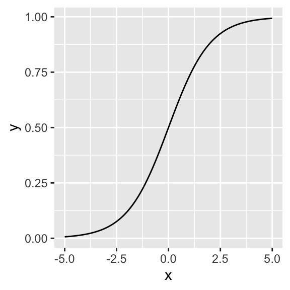

The regression thus can be written as:

\[Pr(infestation = 1) = logit^{−1}(\beta_0 + \beta_1 * temp)) = \frac{1}{1 + e^{-(\beta_0 + \beta_1 * temp)}}\]

In our case the data is binomially distributed. Hence, we can relate the probability of infestation modelled through the logit-link to our data using a binomial distribution with one trial, which translates into the Bernoulli distribution (a special case of the binomial distribution with only one trial):

\[infestation \sim Bernoulli(logit^{−1}(\beta_0 + \beta_1 * temp))\]

This model is called binomial logistic regression, there are also multinomial (three or more outcomes) and ordinal logistic regression (ordinal outcomes).

Fitting a logistic regression model to our data:

infested.bin <- glm(infested ~ temp_anomaly, data = dat, family = binomial(link = "logit"))

And plotting the regression line:

prediction <- data.frame(temp_anomaly = seq(-2, 2, length.out = 100))
prediction$fitted <- predict(object = infested.bin, newdata = prediction, type = "response")

ggplot() +
  geom_point(data = dat, aes(x = temp_anomaly, y = infested)) +
  geom_line(data = prediction, aes(x = temp_anomaly, y = fitted))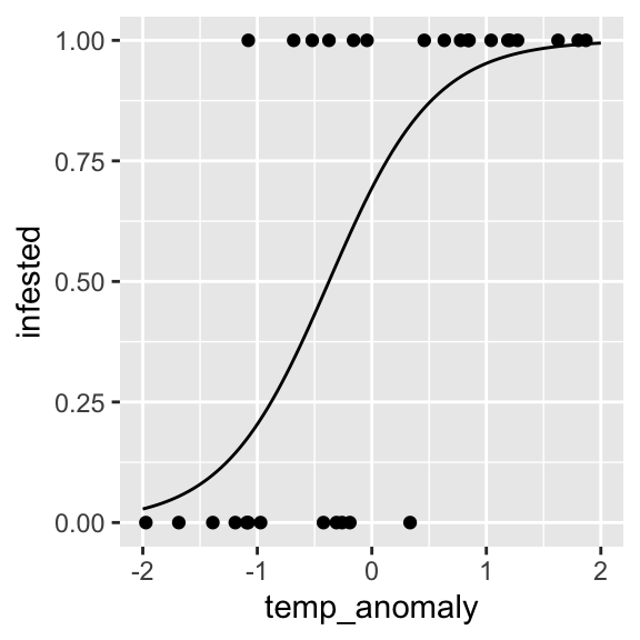

Confidence intervals

To calculate the confidence intervals, we have to first calculate them on the link-scale and then back-transform (plogis) them onto the predictor scale:

pred <- predict(object = infested.bin, newdata = prediction, 
                type = "link", se.fit = TRUE)

prediction$fitted_link <- pred$fit
prediction$lower_link <- prediction$fitted_link - 2 * pred$se.fit
prediction$upper_link <- prediction$fitted_link + 2 * pred$se.fit

prediction$link <- plogis(prediction$fitted_link)
prediction$lower <- plogis(prediction$lower_link)
prediction$upper <- plogis(prediction$upper_link)

And add them to the plot:

ggplot() +
  geom_point(data = dat, aes(x = temp_anomaly, y = infested)) +
  geom_ribbon(data = prediction, aes(x = temp_anomaly, ymin = lower, ymax = upper), alpha = 0.3) +
  geom_line(data = prediction, aes(x = temp_anomaly, y = fitted))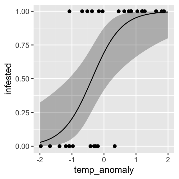

`effects` package

Alternatively, we can use the effect() function, which does the transformation automatically:

library(effects)

efct <- effect("temp_anomaly", 
               mod = infested.bin, 
               xlevels = list(temp_anomaly = seq(-2, 2, length.out = 100)))
efct <- as.data.frame(efct)

ggplot() +
  geom_point(data = dat, aes(x = temp_anomaly, y = infested)) +
  geom_ribbon(data = efct, aes(x = temp_anomaly, ymin = lower, ymax = upper), alpha = 0.3) +
  geom_line(data = efct, aes(x = temp_anomaly, y = fit))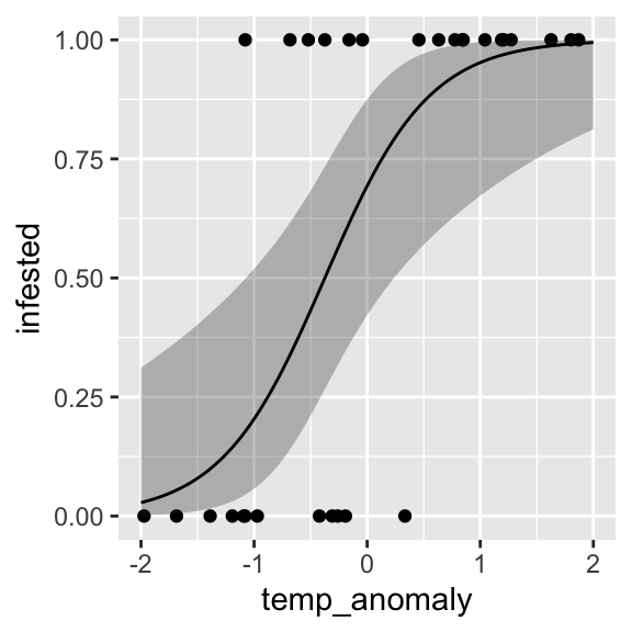

`dose.p()`

We can estimate the temperature anomaly value at which the infestation probability is 50% using dose.p() from the MASS package.

library(MASS)
temp_anomaly_p50 <- dose.p(infested.bin, p=0.5)
temp_anomaly_p50

##                Dose        SE
## p = 0.5: -0.3744093 0.2372779

ggplot() +
  geom_point(data = dat, aes(x = temp_anomaly, y = infested)) +
  geom_vline(xintercept=temp_anomaly_p50) +
  geom_line(data = prediction, aes(x = temp_anomaly, y = fitted))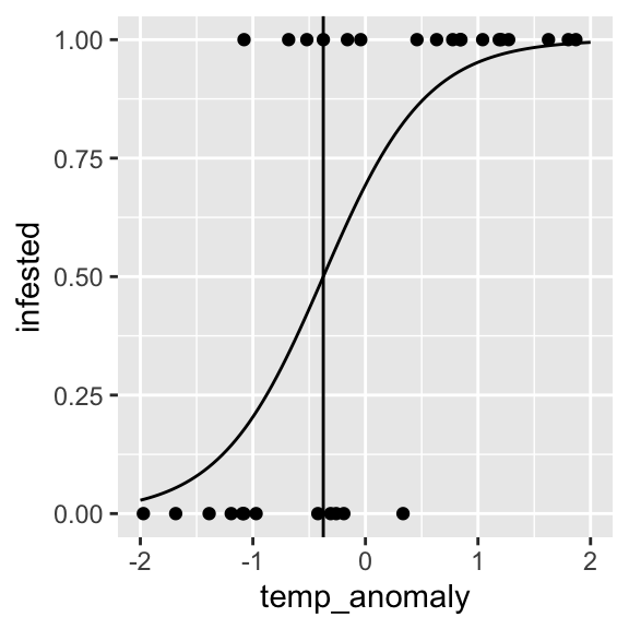

Interpretation

It is not straightforward to interpret coefficients in logistic regression, because the change in y given a unit change in x is non-linear (though linear on the link scale!). However, there are - besides plotting - some ways of making the regression coefficients interpretable.

The divide by 4 rule uses the fact that the logistic curve is steepest at its center (which is at zero given scaled predictors).

As a rough estimate, we can take logistic regression coefficients and divide them by 4 to get an upper bound of the predictive difference corresponding to a unit difference in x. This upper bound is a good approximation near the midpoint of the logistic curve, where probabilities are close to 0.5.

In the our example, the regression coefficient was 2.18. Dividing 2.18 by 4 yields 0.54. We can thus say that with an increase in temperature anomaly by one standard deviation, there is an expected increase in infestation probability by no more than 54%.

summary(infested.bin)

## 
## Call:
## glm(formula = infested ~ temp_anomaly, family = binomial(link = "logit"), 
##     data = dat)
## 
## Coefficients:
##              Estimate Std. Error z value Pr(>|z|)   
## (Intercept)    0.8154     0.5766   1.414  0.15734   
## temp_anomaly   2.1778     0.7809   2.789  0.00529 **
## ---
## Signif. codes:  0 '***' 0.001 '**' 0.01 '*' 0.05 '.' 0.1 ' ' 1
## 
## (Dispersion parameter for binomial family taken to be 1)
## 
##     Null deviance: 40.381  on 29  degrees of freedom
## Residual deviance: 23.488  on 28  degrees of freedom
## AIC: 27.488
## 
## Number of Fisher Scoring iterations: 5

Odds ratios

Another way to interpret logistic regression coefficients is in terms of odds ratios.

If a success has the probability \(p\) and failure the probability \((1 − p)\), then \(p/(1 − p)\) is called the odds. Thus, the odds of success are defined as the ratio of the probability of success over the probability of failure.

An odds of 1 is equivalent to a probability of 0.5, that is equally likely outcomes (1:1). An odds of 0.5 is equivalent to a probability of 0.33, indicating there is a 1:2 chance of success. An odds of 2 is equivalent to a probability of 0.66, indicating a 2:1 chance of success.

The ratio of two odds is called an odds ratio: \(\frac{p_1/(1 − p_1)}{p_2/(1 − p_2)}\).
The odds ratio indicates the preference of outcome A over outcome B.

Example

We observed a plant species in 6 out of 10 plots in landscape A and in 4 out of 10 plots in landscape B.
This gives us probabilities of 0.6 and 0.4. The odds ratio of observing the plant in landscape A over observing it in landscape B is \(\frac{0.6/0.4}{0.4/0.6} = 2.25\).
Hence, there is a 2.25 times higher chance of observing the plant in landscape A compared to landscape B.
The logistic regression coefficients give the change in log odds (recall the link function \(\log(\frac{p}{1-p})\).
When exponentiated, logistic regression coefficients can be interpreted as odds ratios:

\(\frac{odds(x + 1)}{odds(x)} = \frac{e^{\beta_0 + \beta_1 (x + 1)}}{e^{\beta_0 + \beta_1 x}} = e^{\beta_1}\)

For continuous predictors, the coefficients give the change in the log odds of the outcome for a unit increase in the predictor variable.
For categorical predictors, the coefficient estimate describes the change in the log odds for each level compared to the base level.

Infestation example

Infestation example:

exp(coef(infested.bin)[2])

## temp_anomaly 
##     8.826474

The odds ratio indicates that with a one SD change in temperature anomaly there is a 8.83 times higher chance of infestation over no infestation.

Generalized linear models in R I

Humboldt-Universität zu Berlin | Geography Department

Content

Generalized Linear Models

The `glm` function

Family argument

Extractor functions

From LM to GLM

Advantages

Logistic Regression

Proportions response data

Residual analysis

Binary response data

Confidence intervals

`effects` package

`dose.p()`

Interpretation

Odds ratios

Example

Infestation example

Generalized linear models in R I

Humboldt-Universität zu Berlin | Geography Department

Content

Generalized Linear Models

The glm function

Family argument

Extractor functions

From LM to GLM

Advantages

Logistic Regression

Proportions response data

Residual analysis

Binary response data

Confidence intervals

effects package

dose.p()

Interpretation

Odds ratios

Example

Infestation example

The `glm` function

`effects` package

`dose.p()`