Packages

library(ggplot2) # load ggplot2 package for visualization
library(tidyr) # data wrangling package: change from wide to long format
library(dplyr) # data manipulation: mutate
library(gridExtra) # plot multiple ggplot graphs

Anscombe dataset

The anscombe dataset is shipped with base R. It consists of 4 bivariate datasets: x1:y1, x2:y2, x3:y3, and x4:y4.

data(anscombe) # load anscombe (installed with R)
head(anscombe, 2) # print first two rows

##   x1 x2 x3 x4   y1   y2   y3   y4
## 1 10 10 10  8 8.04 9.14 7.46 6.58
## 2  8  8  8  8 6.95 8.14 6.77 5.76

For this exercise, we will use the first anscombe dataset.

ggplot(anscombe, aes(x = x1, y = y1)) +
       geom_point()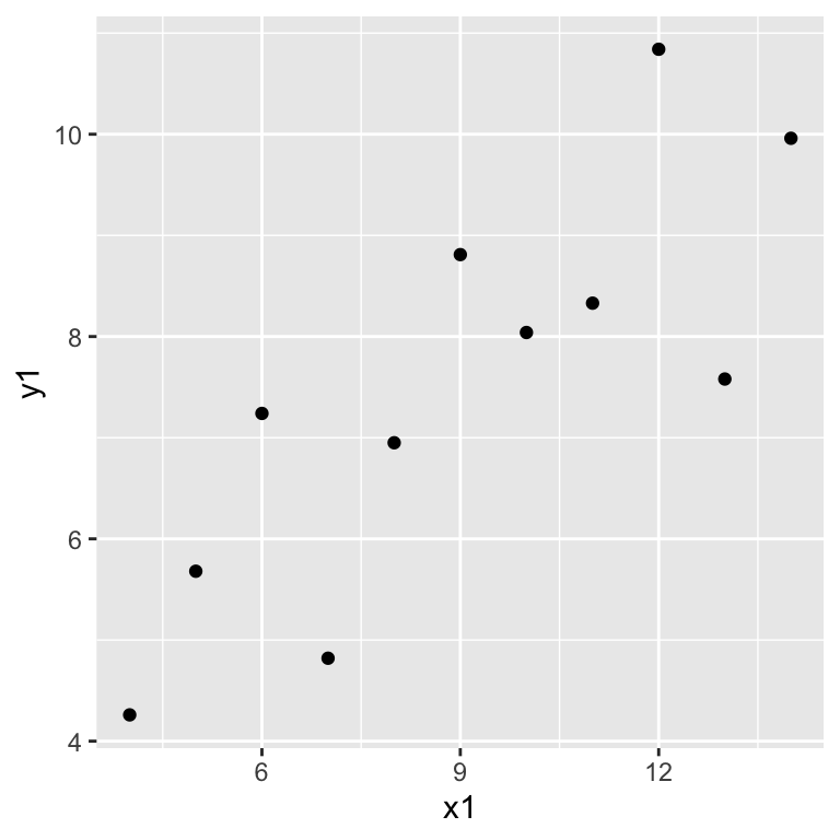

Model fitting with `lm()`

The lm() function implements simple linear regression in R. The argument to lm() is a model formula in which the tilde symbol (~) should be read as “described by”.

lmd.ans1 <- lm(y1 ~ x1, data = anscombe) # fit model
lmd.ans1 # print the lm object lm.ans1

## 
## Call:
## lm(formula = y1 ~ x1, data = anscombe)
## 
## Coefficients:
## (Intercept)           x1  
##      3.0001       0.5001

The result of lm() is a model object. This is a distinctive concept of R. Whereas other statistical systems focus on generating printed output that can be controlled by setting options, you get instead the result of a model fit encapsulated in an object from which the desired quantities can be obtained using extractor functions. Printing the created model object gives you the model formula and the coefficients (intercept and slope). More information about the model can be accessed with extractor functions. We’ll do that later.

Visualization

We can plot the regression line from the estimated slope (\(\beta_{1}\)) and intercept (\(\beta_{0}\)) using geom_abline():

ggplot(anscombe, aes(x = x1, y = y1)) +
  geom_point() +
  geom_abline(intercept = 3.0001, slope = 0.5001, col = "red")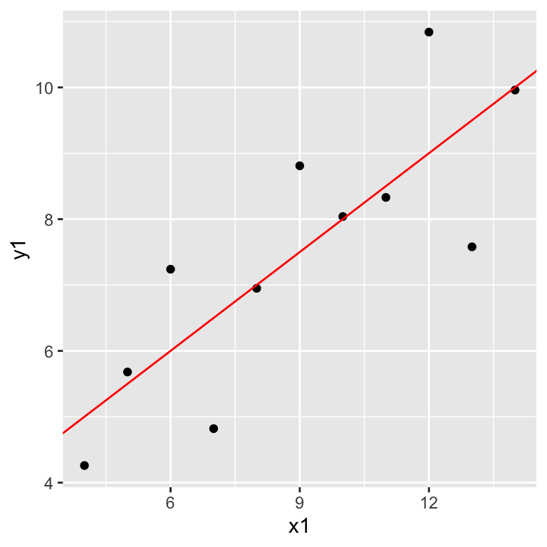

Note, we here typed in the parameter estimates manually (we hardcoded them). It is much more convenient to extract the parameter estimates using the extractor function coefficients(), which we do below.

ANOVA table in R

Calling anova() on an object returned by lm() computes the ANOVA table. The SSE is 13.763, the mean squared error is 1.529 (with 9 degrees of freedom), and the SSR is 27.51.

The value of the F-statistic (\(F_s\)) is 17.99.

anova(lmd.ans1)

## Analysis of Variance Table
## 
## Response: y1
##           Df Sum Sq Mean Sq F value  Pr(>F)   
## x1         1 27.510 27.5100   17.99 0.00217 **
## Residuals  9 13.763  1.5292                   
## ---
## Signif. codes:  0 '***' 0.001 '**' 0.01 '*' 0.05 '.' 0.1 ' ' 1

Note, we can also do the F-test manually by looking up the \(F_s\) value in the F-distribution. Recall, the F-distribution has two parameters: the degrees of freedom of the regression (\(df_1 = 1\)), and the degrees of freedom of the error (\(df_2 = n-2\)).

# p-value of the F-test
1 - pf(17.99, 1, 11-2)

## [1] 0.002169607

As the p-value is very small, we safely reject the null hypothesis \(H_0 : \beta_1 = 0\), indicating a significant effect of \(x\) on \(y\). However, be aware that the p-value does not indicate the effect size! The effect size (change in \(y\) with one unit change in \(x\)) is given by the regression slope (\(\beta_1\)).

Extractor functions

Using the summary() function we can get a more comprehensive summary of the model statistics, including the F-test, t-tests for individual parameters, and coefficient of determination (\(R^2\)).

summary(lmd.ans1)

## 
## Call:
## lm(formula = y1 ~ x1, data = anscombe)
## 
## Residuals:
##      Min       1Q   Median       3Q      Max 
## -1.92127 -0.45577 -0.04136  0.70941  1.83882 
## 
## Coefficients:
##             Estimate Std. Error t value Pr(>|t|)   
## (Intercept)   3.0001     1.1247   2.667  0.02573 * 
## x1            0.5001     0.1179   4.241  0.00217 **
## ---
## Signif. codes:  0 '***' 0.001 '**' 0.01 '*' 0.05 '.' 0.1 ' ' 1
## 
## Residual standard error: 1.237 on 9 degrees of freedom
## Multiple R-squared:  0.6665, Adjusted R-squared:  0.6295 
## F-statistic: 17.99 on 1 and 9 DF,  p-value: 0.00217

The function fitted() returns fitted values \(\hat{y}_i\), i.e., the y-values that you would expect for the given x-values according to the best-fitting straight line. The residuals shown by residuals() are the differences between the observed \(y_i\) and the fitted values: \(y_i-\hat{y}_i\).

fitted(lmd.ans1)

##         1         2         3         4         5         6         7         8 
##  8.001000  7.000818  9.501273  7.500909  8.501091 10.001364  6.000636  5.000455 
##         9        10        11 
##  9.001182  6.500727  5.500545

residuals(lmd.ans1)

##           1           2           3           4           5           6 
##  0.03900000 -0.05081818 -1.92127273  1.30909091 -0.17109091 -0.04136364 
##           7           8           9          10          11 
##  1.23936364 -0.74045455  1.83881818 -1.68072727  0.17945455

The function coefficients() returns the estimated model parameters; in this case intercept and slope.

coefficients(lmd.ans1)

## (Intercept)          x1 
##   3.0000909   0.5000909

You can extract both parameters using simple vector indexing:

intercept <- coefficients(lmd.ans1)[1]
slope <- coefficients(lmd.ans1)[2]

Predicted values can be extracted with the function predict(). With no arguments, it just gives the fitted values:

predict(lmd.ans1) # same as fitted(lmd.ans1)

##         1         2         3         4         5         6         7         8 
##  8.001000  7.000818  9.501273  7.500909  8.501091 10.001364  6.000636  5.000455 
##         9        10        11 
##  9.001182  6.500727  5.500545

You can also predict outcomes for new values. The data frame supplied to newdata must have the same column names that were used in the formula in lm()!

new.ans1 <- data.frame(x1 = c(1, 4, 6, 19))
predict(lmd.ans1, newdata = new.ans1)

##         1         2         3         4 
##  3.500182  5.000455  6.000636 12.501818

Setting the argument interval = "confidence" you get the vector of predicted values with a lower and upper limit given uncertainty in the parameters.

predict(lmd.ans1, interval = 'confidence')

##          fit      lwr       upr
## 1   8.001000 7.116387  8.885613
## 2   7.000818 6.116205  7.885431
## 3   9.501273 8.141258 10.861287
## 4   7.500909 6.657464  8.344354
## 5   8.501091 7.503113  9.499069
## 6  10.001364 8.423422 11.579305
## 7   6.000636 4.838027  7.163245
## 8   5.000455 3.422513  6.578396
## 9   9.001182 7.838573 10.163791
## 10  6.500727 5.502750  7.498705
## 11  5.500545 4.140531  6.860560

Note that R by default returns the 95% confidence interval. You can change this by setting the argument level to another confidence level (e.g., level = 0.99).

Confidence bands

prediction.anscombe1 <- lmd.ans1 %>%
  predict(., interval = 'confidence') %>%
  as.data.frame() %>%
  mutate(x = anscombe$x1)

ggplot(anscombe, aes(x = x1, y = y1)) +
  geom_point() +
  geom_line(data = prediction.anscombe1, aes(x = x, y = fit)) +
  geom_line(data = prediction.anscombe1, aes(x = x, y = upr), linetype = "dashed" ) +
  geom_line(data = prediction.anscombe1, aes(x = x, y = lwr), linetype = "dashed")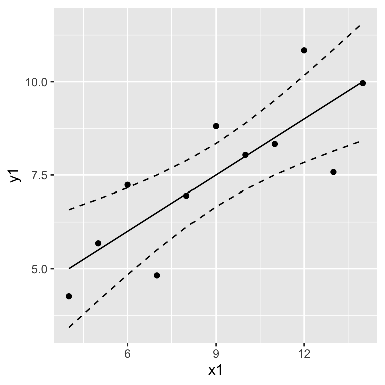

Interpret the confidence band as: When repeating the experiment, we would expect that the estimated regression lines lie within the confidence band 95% of the time.

Prediction bands

If you add interval = "prediction", then you get the vector of predicted values with a lower and upper limit given uncertainty in the parameters plus residual variance.

prediction.anscombe1 <- lmd.ans1 %>%
  predict(., interval = 'prediction') %>%
  as.data.frame() %>%
  mutate(x = anscombe$x1)

## Warning in predict.lm(., interval = "prediction"): predictions on current data refer to _future_ responses

ggplot(anscombe, aes(x = x1, y = y1)) +
  geom_point() +
  geom_line(data = prediction.anscombe1, aes(x = x, y = fit)) +
  geom_line(data = prediction.anscombe1, aes(x = x, y = upr), linetype = "dashed" ) +
  geom_line(data = prediction.anscombe1, aes(x = x, y = lwr), linetype = "dashed")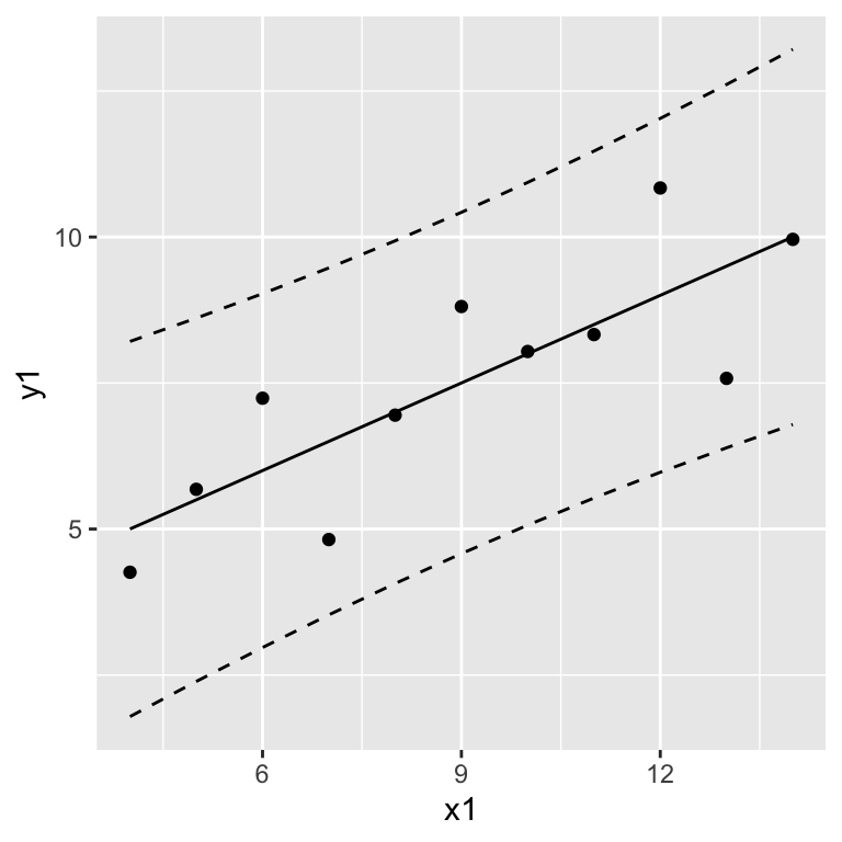

Interpret the prediction band as: When predicting new values, we would expect that 95% of them lie within the prediction band.

Model diagnostics

Five-step plan

The validity of a model depends on several assumptions regarding the distribution of residuals and the functional relationship between \(y\) and \(x\). Visual and numerical model diagnostics should cover the following aspects:

Analysis of the functional relationship between response and predictor
Analysis of the distribution of the predictor variable
Analysis of leverage points (points with high influence)
Analysis of the dispersion of the response
Analysis of the residuals (independence, normal distribution, and homoscedasticity)

Functional relationship

When fitting a linear regression model, we assume a linear relationship between \(y\) and \(x\). But this assumption may be incorrect. To test whether an assumed relationship matches the data or not, you may need to compare different models (including data transformations). You should also apply your mechanistic understanding of the system you are trying to analyse.

# turn into long format
anscombe.long <- mutate(anscombe, id=1:nrow(anscombe)) %>% 
                 pivot_longer(., cols= -id, names_to="key", values_to="value") %>%
                 extract(., key, c("var", "dataset"), "(.)(.)") %>%
                 pivot_wider(., names_from=var, values_from=value)

ggplot(anscombe.long, aes(x = x, y = y)) +
    geom_point(alpha = 0.5) +
    geom_smooth(method = "lm", se = FALSE, col = 'red', lwd = 0.5) +     
    facet_wrap(~dataset, scales = "free", ncol=4)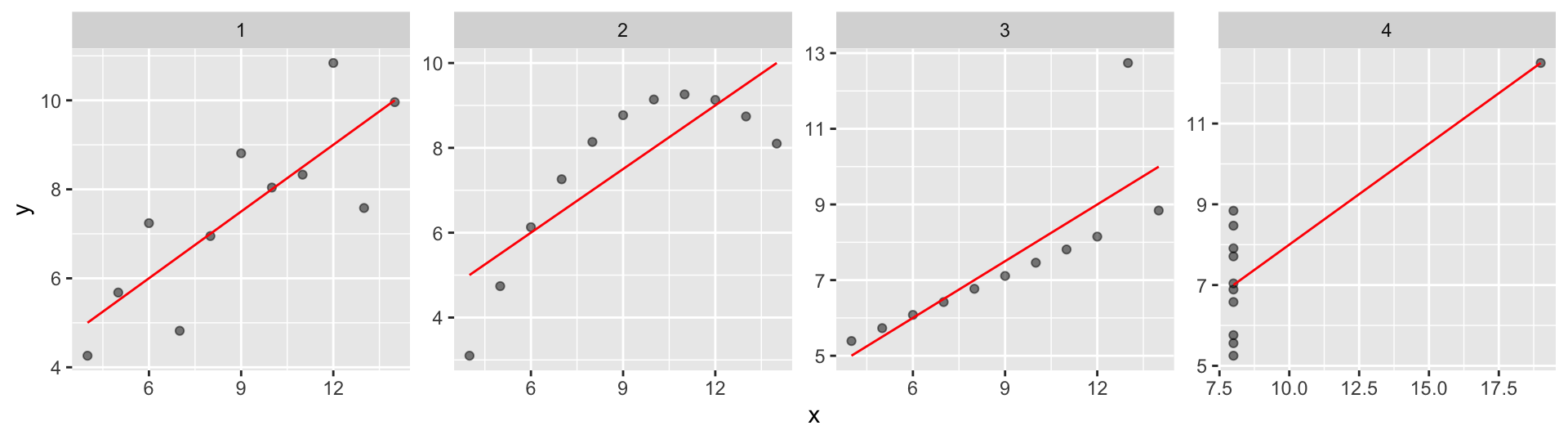

Distribution of predictor

Extreme \(x\) values can dominate a regression.
Ideally, \(x\) would be uniformly distributed. We make no explicit assumptions on the distribution of \(x\), but it can matter.
This should be considered when designing experiments and sampling surveys.
Log- and squareroot-transformations can dampen the effect of extreme values. But be careful as the interpretation changes!

ggplot(anscombe.long, aes(x = dataset, y = x)) +
            geom_boxplot()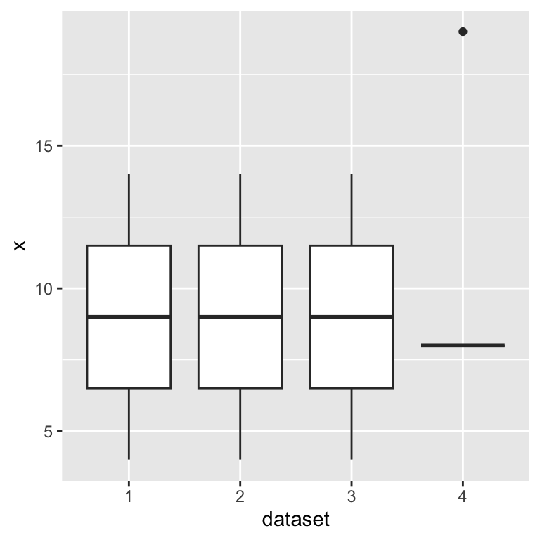

Leverage points

There is no practical justification to eliminate ‘outliers’ just because they are extreme values. Removing extreme values has to be well justified, e.g. by measurement error.

Although, you should not simply delete outliers, you can run your analysis twice (with and without outliers) to test the robustness of the analysis.

Cook’s distance is a common measure to identify influential points. Values greater than 1 or greater than 4/n (n = sample size) are candidate influential points, though we suggest you rely on your intuition rather than strict thresholds. You can extract Cook’s distance using cooks.distance().

Dispersion

Dispersion quantifies how much higher (or lower) the observed variance is relative to the expected variance of the model (overdispersion or underdispersion).
This is often not relevant for the normal distribution case (OLS assumes the residuals to be normally distributed), since the standard deviation (measure of variability) is independent of the mean, and thus estimated separately.
But dispersion will play a role for other distributions modeled with Generalized Linear Models.
…to be continued.

Response residuals

The residuals should be independent of the fitted values. We can check this by plotting the residuals against the fitted values:

lmd.ans1 <- lm(y1 ~ x1, data=anscombe)
anscombe$residuals1 <- residuals(lmd.ans1)
anscombe$fitted1 = fitted(lmd.ans1)

p1 <- ggplot(data = anscombe, aes(x = fitted1, y = residuals1)) +
  geom_point() +
  geom_hline(yintercept = 0, col = "red") +
  labs(title = "Anscombe 1")

lmd.ans2 <- lm(y2 ~ x2, data=anscombe)
anscombe$residuals2 <- residuals(lmd.ans2)
anscombe$fitted2 = fitted(lmd.ans2)

p2 <- ggplot(data = anscombe, aes(x = fitted2, y = residuals2)) +
      geom_point() +
      geom_hline(yintercept = 0, col = "red") +
      labs(title = "Anscombe 2")

gridExtra::grid.arrange(p1, p2, ncol = 2)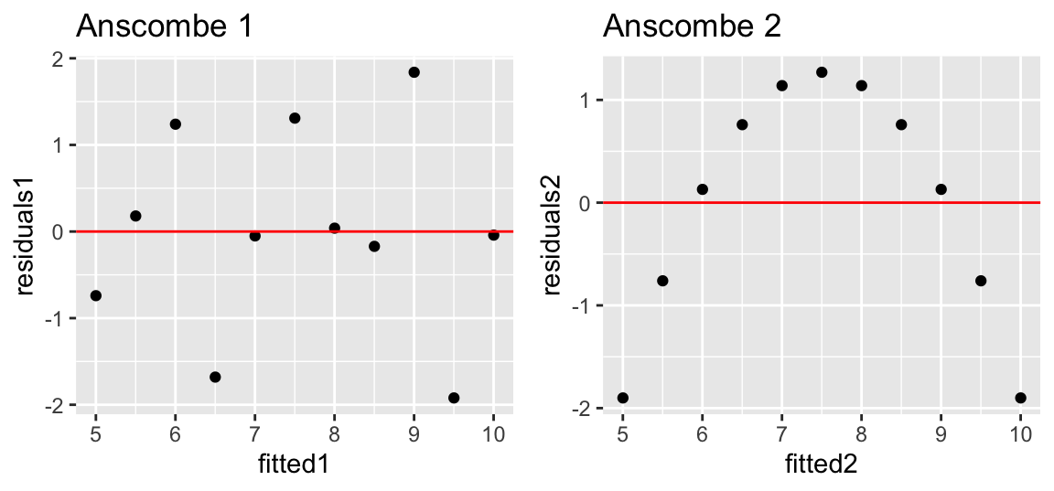

There should be no serial correlation between residuals either. We can check this by plotting the residuals over observations:

p1 <- ggplot(data = anscombe, aes(x=1:11, y = residuals1)) +
  geom_point() +
  geom_hline(yintercept = 0, col = "red") +
  labs(title = "Anscombe 1")


p2 <- ggplot(data = anscombe, aes(x = 1:11, y = residuals2)) +
  geom_point() +
  geom_hline(yintercept = 0, col = "red") +
  labs(title = "Anscombe 2")

gridExtra::grid.arrange(p1, p2, ncol = 2)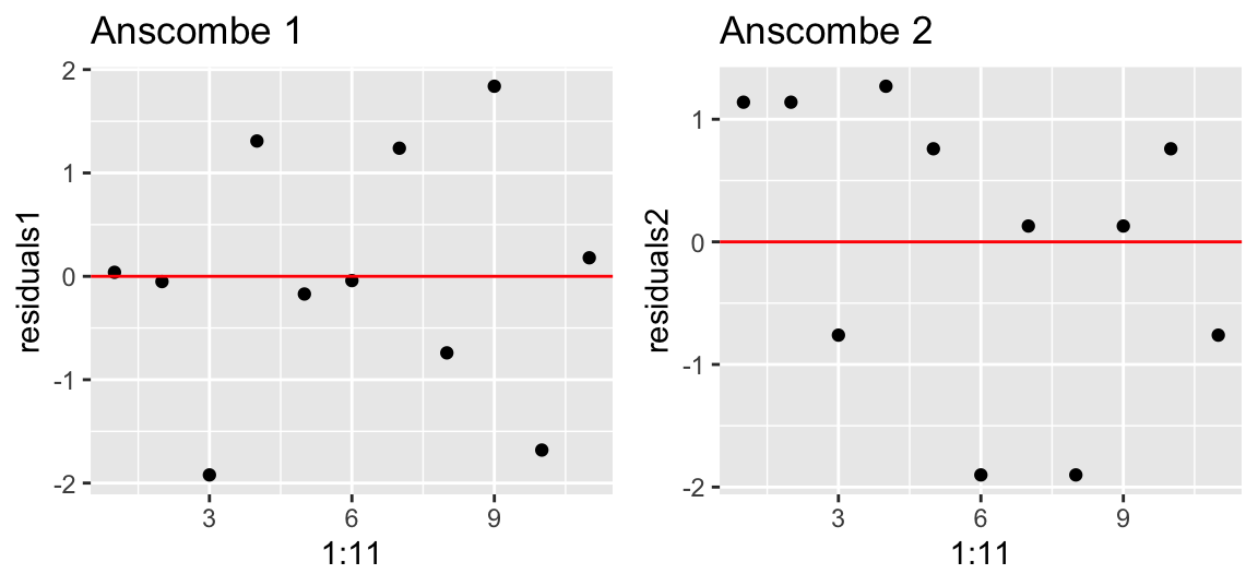

Please note that regression models might have temporally or spatially correlated residuals. In fact, both are very common with ecological data. You will learn how to deal with spatial correlation structures in the residuals later in the course.

The residuals should be normally distributed, which we can test by plotting the residuals via a histogram:

p1 <- ggplot(data = anscombe, aes(x = residuals1)) +
  geom_histogram() +
  labs(title = "Anscombe 1")

p2 <- ggplot(data = anscombe, aes(x = residuals2)) +
  geom_histogram() +
  labs(title = "Anscombe 2")

gridExtra::grid.arrange(p1, p2, ncol = 2)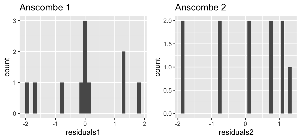

With few data, however, histograms are difficult to assess! Hence, we often prefer QQ-Plots.

The Quantile-Quantile Plot (QQ-Plot) plots the quantiles of the standardized residuals over the corresponding quantiles of a standard normal distribution:

anscombe$resid_standard1 <- rstandard(lmd.ans1) # standardized residuals
p1 <- ggplot(anscombe, aes(sample = resid_standard1)) +
      stat_qq() +
      geom_abline(intercept = 0, slope = 1)

anscombe$resid_standard2 <- rstandard(lmd.ans2) # standardized residuals
p2 <- ggplot(anscombe, aes(sample = resid_standard2)) +
      stat_qq() +
      geom_abline(intercept = 0, slope = 1)

gridExtra::grid.arrange(p1, p2, ncol = 2)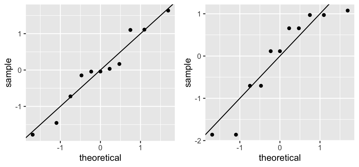

If the two datasets come from the same distribution (the residuals are thus normally distributed), the points should lie roughly on a line through the origin with slope 1. Interpretation takes some experience and is not always easy, especially with small sample sizes. Yet, it is one of the best methods! Try https://xiongge.shinyapps.io/QQplots/ to see the effect of deviations from normality on the QQ-plot.

4. Linear regression in R

Humboldt-Universität zu Berlin | Geography Department

Packages

Anscombe dataset

Model fitting with `lm()`

Visualization

ANOVA table in R

Extractor functions

Confidence bands

Prediction bands

Model diagnostics

Five-step plan

Functional relationship

Distribution of predictor

Leverage points

Dispersion

Response residuals

4. Linear regression in R

Humboldt-Universität zu Berlin | Geography Department

Packages

Anscombe dataset

Model fitting with lm()

Visualization

ANOVA table in R

Extractor functions

Confidence bands

Prediction bands

Model diagnostics

Five-step plan

Functional relationship

Distribution of predictor

Leverage points

Dispersion

Response residuals

Model fitting with `lm()`