Spatial regression in R

---

Overview

In Geography, we are often faced with regression problems that inherently involve geographic locations. The consequences of using locational data potentially are spatial dependence (spatial autocorrelation) and spatial heterogeneity or trends (non-stationarity). In this session, we will focus on statistical problems related to spatial dependence, specifically:

• Diagnose spatial dependence in regression models
• Spatial lag models
• Spatial error models

---

Packages

library(ggplot2)    # Graphics library
library(sf)         # Spatial data types and handling
library(mapview)    # Visualize spatial data
library(spdep)      # Diagnosing spatial dependence
library(spatialreg) # Spatial lag and spatial error model

---

Diagnose spatial dependence

Before testing for spatial dependence, we need to understand the two principal sources of spatial dependence. The first is an explicit interaction between spatial sources: spatial diffusion happens when spatially proximate units are influenced directly by their neighbors, and vice versa. Spatial diffusion effects can be incorporated in spatial lag models by including a spatially lagged response variable as predictor. Second, neighboring units may be similar even if there is no direct exchange or interaction between them. They may be similar just because they share the same underlying process by being geographically clustered. Such spatial dependence may be called attributional dependence because it is related to neighboring locations sharing the same attributes. Sometimes we can account for these attributional sources by including them as explanatory variables in the model (e.g., soil properties, climate). If that doesn’t work, then the model will exhibit spatial dependence in the error terms. Spatial error dependence can be modeled via a spatially lagged error term (spatial error model).

For this exercise, we will use the meuse dataset from last week. Let’s build a simple linear regression model predicting zinc concentration based on elevation and square-root-transformed distance to the river. The question is: are the residuals spatially independent?

meuse <- read_sf('data/meuse.gpkg')

zinc.lm <- lm(log(zinc) ~ elev + sqrt(dist), data = meuse)
summary(zinc.lm)

## 
## Call:
## lm(formula = log(zinc) ~ elev + sqrt(dist), data = meuse)
## 
## Residuals:
##      Min       1Q   Median       3Q      Max 
## -0.99144 -0.22853  0.00209  0.22244  0.98324 
## 
## Coefficients:
##             Estimate Std. Error t value Pr(>|t|)    
## (Intercept)  8.64157    0.25206  34.284  < 2e-16 ***
## elev        -0.23217    0.03426  -6.777 2.54e-10 ***
## sqrt(dist)  -1.97766    0.16025 -12.341  < 2e-16 ***
## ---
## Signif. codes:  0 '***' 0.001 '**' 0.01 '*' 0.05 '.' 0.1 ' ' 1
## 
## Residual standard error: 0.3827 on 152 degrees of freedom
## Multiple R-squared:  0.7226, Adjusted R-squared:  0.7189 
## F-statistic:   198 on 2 and 152 DF,  p-value: < 2.2e-16

meuse$residuals <- residuals(zinc.lm)
meuse$fitted <- fitted(zinc.lm)

# We can plot the location dataset using geom_sf() instead of geom_point()
ggplot(meuse, aes(col = residuals, size = residuals)) +
  geom_sf() +
  scale_color_gradient2()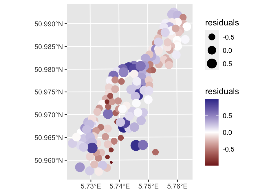

---

Spatial weights

To test for spatial autocorrelation, we first need to identify groups of neighbors. The function dnearneigh identifies neighbors of region points by euclidean distance between lower (greater than) and upper (less than or equal to) bounds. See also knearneigh/knn2nb for k-nearest neighbors and poly2nb for polygon neighborhoods.

meuse.nb <- spdep::dnearneigh(meuse, d1 = 0, d2 = 200)

The result is an nb object, which is a list of vectors. Each vector contains the numerical indices of the observations. For example, the first vector meuse.nb[[1]] contains the indices of the neighbors of the first observation. The first observation has two neighbors: the 2nd and 3rd observation. The second observation has three neighbors: the 1st, 3rd, and 8th observation…

str(meuse.nb, list.len=5, give.attr = F) # show content of first 5 list entries

## List of 155
##  $ : int [1:2] 2 3
##  $ : int [1:3] 1 3 8
##  $ : int [1:4] 1 2 4 7
##  $ : int [1:3] 3 5 7
##  $ : int [1:4] 4 6 7 10
##   [list output truncated]

Next, we need to assign weights to each neighbor with the nb2listw function. In our example, each neighboring sample (point/polygon) is assigned equal weight (style="W"). This is accomplished by assigning the fraction 1/ (# of neighbors) to each neighboring sample.

meuse.lw <- nb2listw(meuse.nb, style = "W", zero.policy = TRUE)

The result is a listw object that contains the neighbor indices (meuse.lw$neighbours) and the corresponding neighbor weights (meuse.lw$weights). The zero.policy=TRUE option allows for lists of non-neighbors. This should be used with caution since the user may not be aware of missing neighbors in their dataset however, a zero.policy of FALSE would return an error.

str(meuse.lw$weights, list.len=5, give.attr = F) 

## List of 155
##  $ : num [1:2] 0.5 0.5
##  $ : num [1:3] 0.333 0.333 0.333
##  $ : num [1:4] 0.25 0.25 0.25 0.25
##  $ : num [1:3] 0.333 0.333 0.333
##  $ : num [1:4] 0.25 0.25 0.25 0.25
##   [list output truncated]

---

Moran I test

The Moran I test statistic for spatial autocorrelation applied to regression residuals is implemented by the function lm.morantest. This function operates on an lm object and requires that a spatial weights object be specified. The tests for spatial correlation requires a listw object, which contains the spatial weights. Since, our listw object meuse.lw contains vectors with no neighbors, we need to select here also the zero.policy option.Note, the usual Moran I test for spatial dependence does not work here. For spatial dependence testing of residuals you need to use the test presented here.

lm.morantest(zinc.lm, meuse.lw, zero.policy = T)

## 
##  Global Moran I for regression residuals
## 
## data:  
## model: lm(formula = log(zinc) ~ elev + sqrt(dist), data = meuse)
## weights: meuse.lw
## 
## Moran I statistic standard deviate = 6.7153, p-value = 9.385e-12
## alternative hypothesis: greater
## sample estimates:
## Observed Moran I      Expectation         Variance 
##      0.415342780     -0.013332733      0.004075003

The Moran I test indicates spatially autocorrelated on the regression residuals (p < 0.001).

---

Rao’s score test

The Moran’s I test statistic has high power against a range of spatial alternatives. However, it does not provide much help in terms of which alternative model would be most appropriate. The Rao’s score test (also called Lagrange Multiplier test) statistics allow a distinction between spatial error models and spatial lag models.

It appears the spatial error term is statistically significant (p < 0.01), whereas and the spatial lag term is not (p = 0.117). This suggests, the spatial error model is more appropriate than the spatial lag model.

lm.RStests(zinc.lm, meuse.lw, test="RSerr", zero.policy = T) # spatial error

## 
##  Rao's score (a.k.a Lagrange multiplier) diagnostics for spatial dependence
## 
## data:  
## model: lm(formula = log(zinc) ~ elev + sqrt(dist), data = meuse)
## test weights: meuse.lw
## 
## RSerr = 43.733, df = 1, p-value = 3.764e-11

lm.RStests(zinc.lm, meuse.lw, test="RSlag", zero.policy = T) # spatial lag model

## 
##  Rao's score (a.k.a Lagrange multiplier) diagnostics for spatial dependence
## 
## data:  
## model: lm(formula = log(zinc) ~ elev + sqrt(dist), data = meuse)
## test weights: meuse.lw
## 
## RSlag = 2.4563, df = 1, p-value = 0.1171

---

Understanding Moran I

Spatially lagged values

Using the information on which observation belongs to which neighborhood, we can compute the average zinc residuals of the neighborhood for each sample and plot them against the (global) residuals of the linear model.

Inc.lag <- lag.listw(meuse.lw, meuse$residuals, zero.policy = T)
plot(meuse$residuals, Inc.lag)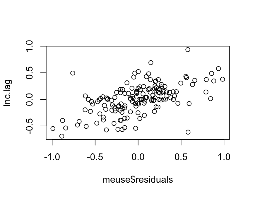

The scatterplot reveals spatial patterns in the residuals: the localized residuals tend to be smaller for negative residuals and higher for positive residuals. You can also use moran.plot to plot the spatially lagged values.

moran.plot(meuse$residuals, meuse.lw, zero.policy = TRUE)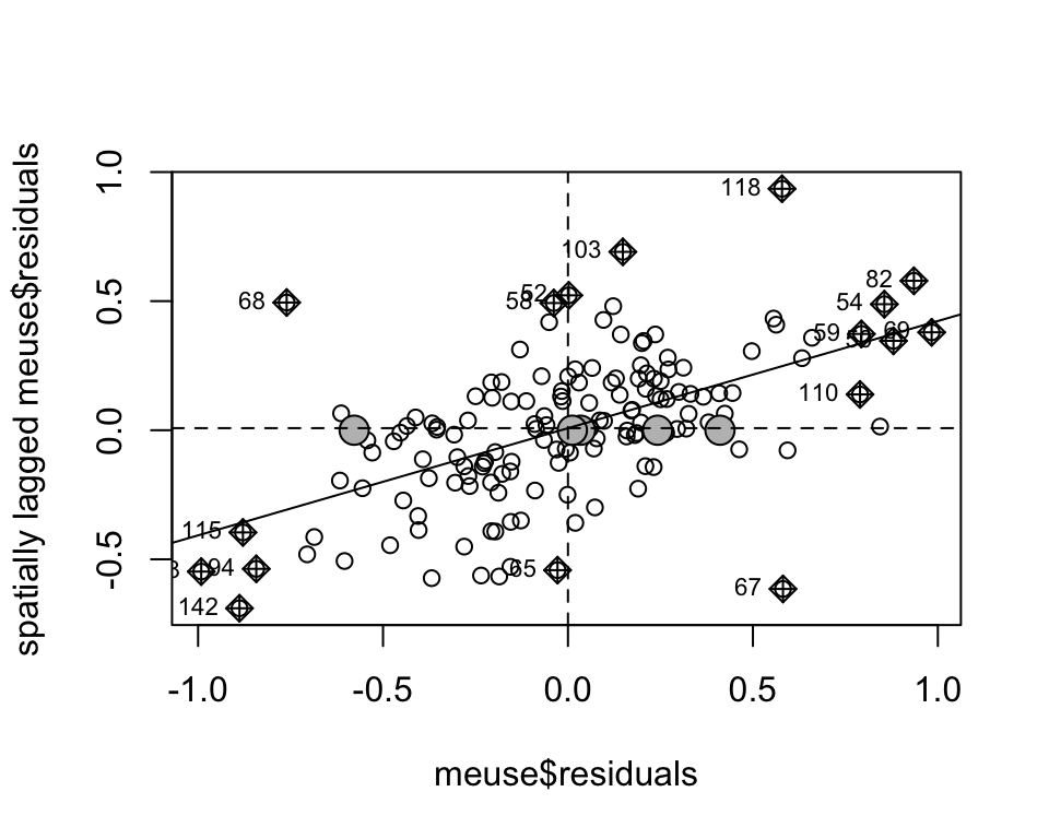

Moran’s I is the slope of the regression line between the spatially lagged values and the observed values (0.415343).

lm(Inc.lag ~ meuse$residuals)

## 
## Call:
## lm(formula = Inc.lag ~ meuse$residuals)
## 
## Coefficients:
##     (Intercept)  meuse$residuals  
##        0.008047         0.415343

---

Monte-carlo simulation

• To assess if the slope is significantly different from zero, we can randomly permute the zinc values across all samples (i.e. we are not imposing any spatial autocorrelation structure).

• Then fit a regression model to each permuted set of values.

• The slope values from the regression give us the distribution of Moran’s I values we could expect to get under the null hypothesis that zinc values are randomly distributed across samples.

• We can then compare the observed Moran’s I value to this distribution.

To test for significance using the monte-carlo simulation method, you can use the moran.mc function.

moran <- moran.mc(meuse$residuals, meuse.lw, nsim = 999, zero.policy = TRUE)
moran

## 
##  Monte-Carlo simulation of Moran I
## 
## data:  meuse$residuals 
## weights: meuse.lw  
## number of simulations + 1: 1000 
## 
## statistic = 0.41534, observed rank = 1000, p-value = 0.001
## alternative hypothesis: greater

The Moran I test statistic of 0.41534 is significantly higher than the 1000 simulated Moran I statistics calculated on random data (p = 0.001). The plot below illustrates the density distribution of the simulated Moran test and the observed Moran test statistic (black vertical line).

plot(moran, main="", las=1)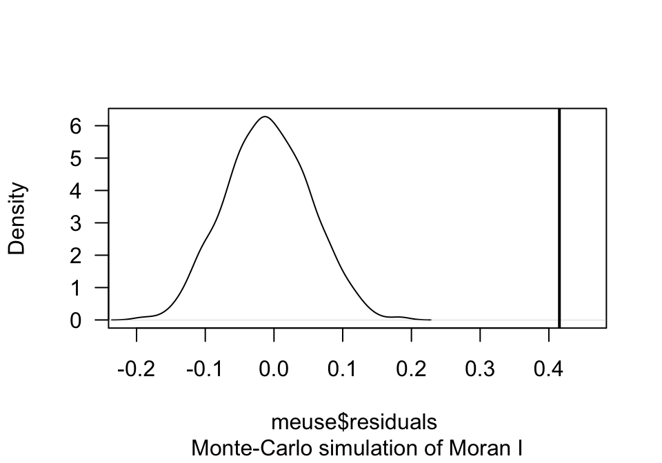

---

Sensitivity analysis

Spatial autocorrelation is scale depended, i.e. the size of the neighborhood. We can assess how spatial autocorrelation (Moran’s I) changes with the upper size limit of the neighborhood (d2):

# empty vector for storage of Moran's I values
moran_I <- c()

# loop d through a sequence ranging from 50 to 2000
for (d in seq(50, 2000, 50)) {
  meuse.nb <- dnearneigh(meuse, d1 = 0, d2 = d)
  meuse.lw <- nb2listw(meuse.nb, style = "W", zero.policy = TRUE)
  moran <- moran.mc(zinc.lm$residuals, meuse.lw, nsim = 999, zero.policy = TRUE)
  moran_I <- c(moran_I, moran$statistic)
}

moran_I <- data.frame(moran = moran_I, 
                      distance = seq(50, 2000, 50))

ggplot(moran_I, aes(x = distance, y = moran)) + 
  geom_point() +
  geom_line()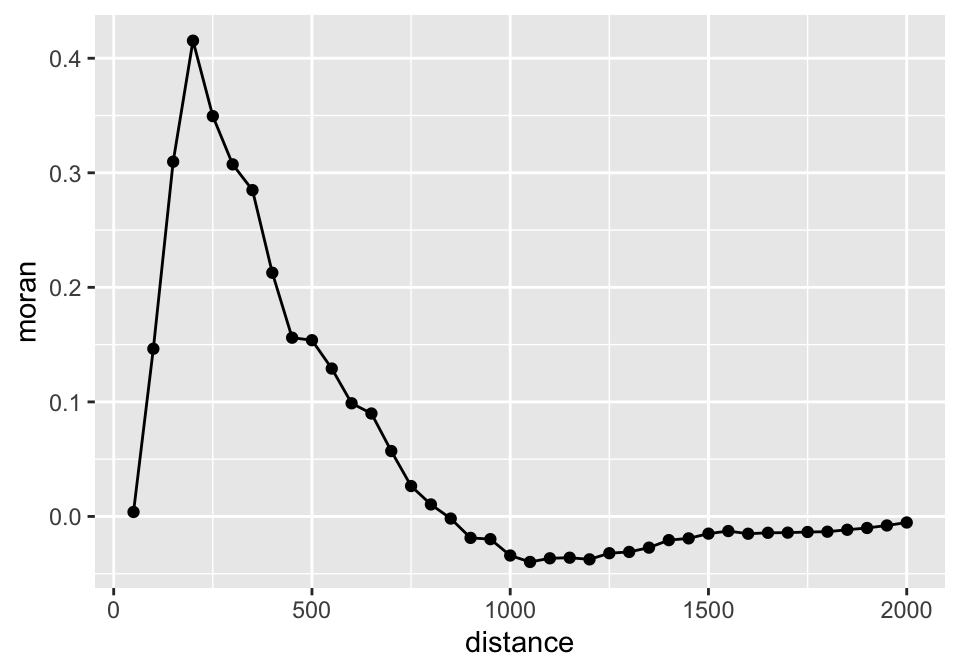

Spatial autocorrelation increases up to 250 m distance. Then autocorrelation decreases until it reaches low values at around 750 m distance.

---

Spatial lag model

We can use spatial lag models (or spatial simultaneous autoregressive lag model) to deal with spatial auto-correlation in the residuals. Spatial lag models include a term (\(\rho W\)) for the spatial autocorrelation in the response variable (\(Y\)):

\(Y = \rho W Y + X\beta + \epsilon\)

where \(\rho\) estimates the influence of neighboring values of \(Y\). \(W\) defines the spatial weights of the neighborhood. For the error term, we assume \(\epsilon \sim N(0, \sigma)\).

Maximum Likelihood (ML) estimation of the spatial lag model is carried out with the lagsarlm() function from the spatialreg package. The required arguments are a regression formula, a data set and a listw spatial weights object.

# define spatial neighborhoods - nb object
meuse.nb <- dnearneigh(meuse, d1 = 0, d2 = 200)

# define spatial weights for neighborhoods - listw object
meuse.lw <- nb2listw(meuse.nb, style = "W", zero.policy = TRUE)

# fit spatial lag moddel
zinc.slm <- lagsarlm(log(zinc) ~ elev + sqrt(dist), data = meuse, listw = meuse.lw, zero.policy = TRUE)

Confirming the Lagrange Multiplier test, the spatial autoregressive parameter \(\rho\) (Rho) is not significant as indicated by the Likelihood Ratio test (p = 0.11829) and the asymptotic t-test (p = 0.11907). The Likelihood Ratio (LR) test is a test of the model with and without the spatial lag. Hence, the reported LR test suggests that the addition of the lag is not an improvement.

## 
## Call:lagsarlm(formula = log(zinc) ~ elev + sqrt(dist), data = meuse, 
##     listw = meuse.lw, zero.policy = TRUE)
## 
## Residuals:
##        Min         1Q     Median         3Q        Max 
## -0.9711349 -0.2303691 -0.0042542  0.2166367  0.9730583 
## 
## Type: lag 
## Regions with no neighbours included:
##  30 106 108 148 155 
## Coefficients: (asymptotic standard errors) 
##              Estimate Std. Error  z value  Pr(>|z|)
## (Intercept)  8.311927   0.329561  25.2212 < 2.2e-16
## elev        -0.228186   0.033823  -6.7465 1.515e-11
## sqrt(dist)  -1.879407   0.168725 -11.1388 < 2.2e-16
## 
## Rho: 0.044484, LR test value: 2.4399, p-value: 0.11829
## Asymptotic standard error: 0.028539
##     z-value: 1.5587, p-value: 0.11907
## Wald statistic: 2.4295, p-value: 0.11907
## 
## Log likelihood: -68.32293 for lag model
## ML residual variance (sigma squared): 0.1413, (sigma: 0.3759)
## Number of observations: 155 
## Number of parameters estimated: 5 
## AIC: 146.65, (AIC for lm: 147.09)
## LM test for residual autocorrelation
## test value: 39.746, p-value: 2.893e-10

---

Spatial error model

The spatial lag model did not improve our spatially auto-correlated residuals. Alternatively, we can use a spatial error model, which assumes that the autoregressive process occurs in the error term (not in the response \(Y\)):

\(Y = X\beta + \lambda W \mu + \epsilon\)

where \(\lambda\) is the spatial autoregression coefficient, \(W\) is the spatial weights matrix, and \(\mu\) the spatial error term.

ML estimation of the spatial error model is similar to the lag procedure and implemented in the errorsarlm() function from the spatialreg package. Again, the formula, data set and a listw spatial weights object must be specified, as illustrated below.

# define spatial neighborhoods - nb object
meuse.nb <- dnearneigh(meuse, d1 = 0, d2 = 200)

# define spatial weights for neighborhoods - listw object
meuse.lw <- nb2listw(meuse.nb, style = "W", zero.policy = TRUE)

zinc.sem <- errorsarlm(log(zinc) ~ elev + sqrt(dist), data = meuse, listw = meuse.lw, zero.policy = TRUE)

The estimate for the spatial autoregressive coefficient \(\lambda\) (Lambda) is significant, which confirms the Lagrange Multiplier test conducted before.

## 
## Call:errorsarlm(formula = log(zinc) ~ elev + sqrt(dist), data = meuse, 
##     listw = meuse.lw, zero.policy = TRUE)
## 
## Residuals:
##      Min       1Q   Median       3Q      Max 
## -1.03979 -0.19864  0.02663  0.19649  0.85387 
## 
## Type: error 
## Regions with no neighbours included:
##  30 106 108 148 155 
## Coefficients: (asymptotic standard errors) 
##              Estimate Std. Error z value  Pr(>|z|)
## (Intercept)  8.757203   0.239257 36.6016 < 2.2e-16
## elev        -0.250525   0.031123 -8.0494 8.882e-16
## sqrt(dist)  -1.912453   0.193397 -9.8887 < 2.2e-16
## 
## Lambda: 0.51114, LR test value: 38.267, p-value: 6.1697e-10
## Asymptotic standard error: 0.073506
##     z-value: 6.9537, p-value: 3.5594e-12
## Wald statistic: 48.353, p-value: 3.5593e-12
## 
## Log likelihood: -50.40936 for error model
## ML residual variance (sigma squared): 0.10296, (sigma: 0.32087)
## Number of observations: 155 
## Number of parameters estimated: 5 
## AIC: 110.82, (AIC for lm: 147.09)

---

Model comparison

In our example, the test statistics clearly speak in favor of the spatial error model, but that may not always be the case. It may happen that both models are significant. A direct comparison between the two models can be based on the maximized log-likelihood (not on measures of fit such as \(R^2\)). In our example, the log-likelihood for the error model of -50.40936 is better (higher) than the one for the lag model of -68.32293. However, the actual values are not that meaningful and the difference between the likelihoods cannot be compared more formally in a LR test because the two models are non-nested (that is, one cannot be obtained from the other by setting coefficients or functions of coefficients to zero).

We may compare the models based on the AIC. The lag model zinc.slm only slightly reduces the AIC compared to the non-spatial linear model zinc.lm. In comparison, the spatial error model zinc.sem has a substantially lower AIC, suggesting that it is the best model among the three.

AIC(zinc.lm, zinc.slm, zinc.sem)

##          df      AIC
## zinc.lm   4 147.0857
## zinc.slm  5 146.6459
## zinc.sem  5 110.8187

Below we compare how the two models reduce the spatial autocorrelation (at different neighborhood sizes) using the Moran I test on the residuals. The graph shows that only the spatial error model reduces the spatial autocorrelation in the residuals effectively.

# create empty vectors for holding the Moran statistics
moran_I_lm <- c()
moran_I_slm <- c()
moran_I_sem <- c()

# loop through a distance vector d ranging from 50 to 2000 m
for (d in seq(50, 2000, 50)) {
  meuse.nb <- dnearneigh(meuse, d1 = 0, d2 = d)
  meuse.lw <- nb2listw(meuse.nb, style = "W", zero.policy = TRUE)
  
  moran_lm <- moran.mc(zinc.lm$residuals, meuse.lw, nsim = 999, zero.policy = TRUE)
  moran_I_lm <- c(moran_I_lm, moran_lm$statistic)
  
  moran_slm <- moran.mc(zinc.slm$residuals, meuse.lw, nsim = 999, zero.policy = TRUE)
  moran_I_slm <- c(moran_I_slm, moran_slm$statistic)
  
  moran_sem <- moran.mc(zinc.sem$residuals, meuse.lw, nsim = 999, zero.policy = TRUE)
  moran_I_sem <- c(moran_I_sem, moran_sem$statistic)
}

moran_I_lm  <- data.frame(moran_I = moran_I_lm, 
                          distance = seq(50, 2000, 50), 
                          model="Simple linear model")

moran_I_slm <- data.frame(moran_I = moran_I_slm, 
                          distance = seq(50, 2000, 50), 
                          model="Spatial lag model")

moran_I_sem <- data.frame(moran_I = moran_I_sem, 
                          distance = seq(50, 2000, 50), 
                          model="Spatial error model")

moran.df <- rbind(moran_I_lm, moran_I_slm, moran_I_sem)
      
ggplot(moran.df, aes(x = distance, y = moran_I, col=model)) + 
  geom_point() +
  geom_line()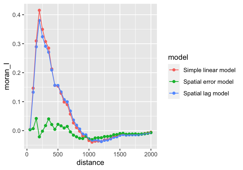

---

References

Anselin, L. (2003). An Introduction to Spatial Regression Analysis in R.

Beale, C.M., Lennon, J.J., Yearsley, J.M., Brewer, M.J., & Elston, D.A. (2010). Regression analysis of spatial data. Ecology Letters, 13, 246-264

Dormann, C.F., M. McPherson, J., B. Araújo, M., Bivand, R., Bolliger, J., Carl, G., G. Davies, R., Hirzel, A., Jetz, W., Daniel Kissling, W., Kühn, I., Ohlemüller, R., R. Peres-Neto, P., Reineking, B., Schröder, B., M. Schurr, F., & Wilson, R. (2007). Methods to account for spatial autocorrelation in the analysis of species distributional data: a review. Ecography, 30, 609-628

Hawkins, B.A. (2012). Eight (and a half) deadly sins of spatial analysis. Journal of Biogeography, 39, 1-9

Copyright © 2024 Humboldt-Universität zu Berlin. Department of Geography.